Data Model¶

There are two types of data, one describing the optical properties of the sample and the second describing the electro-magnetic field of the in-going and out-going light. We will call the first one an optical data and the second one a field data. But first, let us define the coordinate system, units and conventions.

Coordinate system, units and conventions¶

Wavelengths are defined in nanometers.
Dimensions (coordinates) are defined in pixel units.
In the computations, size of the pixel is defined as a parameter (in nanometers).
Optical parameters (orientation of the optical axis) are defined relative to the reference laboratory coordinate frame xyz.
Propagation is said to be forward propagation if the wave vector has a positive z component.
Propagation is said to be backward propagation if the the wave vector has a negative z component.
Light enters the material at z=0 at the bottom of the sample and exits at the top of the sample.
The sample is defined by a sequence of layers - a stack. The first layer is the one at the bottom of the stack.
Internally, optical parameters are stored in memory as a C-contiguous array with axes (i,j,k,…) the axes are z, y, x, parameter(s).

For uniaxial material, the orientation of the optical axis is defined with two angles. $\theta_m$ is an angle between the z axis and the optical axis and $\phi_m$ is an angle between the projection of the optical axis vector on the xy plane and the x axis.

For biaxial media, there is an additional parameter $\psi_m$ that together with $\theta_m$ phi_m` define the three Euler angles for rotations of the frame around the z,y and z axes respectively.

Direction of light propagation (wave vector) is defined with two parameters, $\beta_x = n \sin\theta_k \cos\phi_k$ and $\beta_y = n \sin\theta_k \sin\phi_k$ , or equivalently $\beta = \sqrt{\beta_x^2 + \beta_y^2} = n \sin\theta_k$ and $\phi_k = \arctan(\beta_y/\beta_x)$ , where $\theta_k$ is an angle between the wave vector and the z axis, and $\phi_k$ between the projection of the wave vector on the xy plane and the x axis.

Parameter $\beta$ is a fundamental parameter in transfer matrix method. This parameter is conserved when light is propagated through a stack of homogeneous layers.

Optical Data¶

>>> import dtmm
>>> optical_data = dtmm.nematic_droplet_data((60, 128, 128),
...    radius = 30, profile = "r", no = 1.5, ne = 1.6, nhost = 1.5)

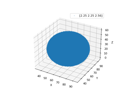
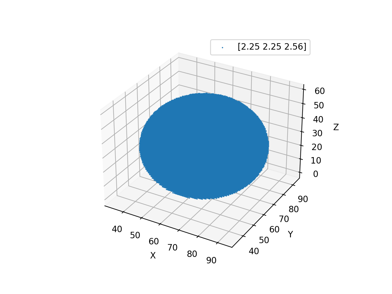
Here we have generated some test optical data, a nematic droplet with a radius of 30 pixels placed in a bounding box of shape (60,128,128), that is, 60 layers of (height - y, width - x) of (128,128). Director profile is radial, with ordinary refractive index of 1.5 and extraordinary refractive index of 1.6 placed in an isotropic host with refractive index of 1.5. The optical data is a tuple of three arrays

>>> thickness, material_eps, eps_angles = optical_data

thickness describes the thickness of layers in the optical data. It is an array of floats. It is measured in pixel units. In our case it is an array of ones of length 60:

>>> import numpy as np
>>> np.allclose(thickness, np.ones(shape = (60,)))
True

which means that layer thickness is the same as layer pixel size - a cubic lattice. Note that in general, layer thickness may not be constant and you can set any layer thickness. material_eps is an array of shape (60,128,128,3) of dtype “float32” or “float64” and describes the three eigenvalues of the dielectric tensor of the material. In our case we have two types of material, a host material (the one surrounding the droplet), and a liquid crystal material. We can plot this data:

>>> fig, ax = dtmm.plot_material(material_eps, dtmm.refind2eps([1.5,1.5,1.6]))
>>> fig.show()

which plots dots at positions where liquid_crystal is defined (where the refractive indices are [1.5,1.5,1.6]). This plots a sphere centered in the center of the bounding box, as shown in Fig.

Fig. 3 LC is defined in a sphere . (Source code, png, hires.png, pdf)¶

material_eps is an array of shape (60,128,128,3). Material is defined by three real (or complex) dielectric tensor eigenvalues (refractive indices squared):

>>> material_eps[0,0,0]
array([2.25, 2.25, 2.25])
>>> material_eps[30,64,64]
array([2.25, 2.25, 2.56])

The real part of the dielectric constant is the refractive index squared and the imaginary part determines absorption properties.

eps_angles is an array of shape (60,128,128,3) and describe optical axis angles measured in radians in voxel. For isotropic material these are all meaningless and are zero, so outside of the sphere, these are all zero:

>>> eps_angles[0,0,0]
array([0., 0., 0.])

while inside of the sphere, these three elements are

>>> eps_angles[30,64,64] #z=30, y = 64, x = 64
array([0.        , 0.95531662, 0.78539816])

The first element is always 0 because it defines the $\psi_m$ angle (used in biaxial materials), the second value describes the $\theta_m$ angle, and the last describes the $\phi_m$ angle.

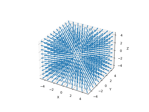
We can plot the director around the center (around the point defect) of the droplet by

>>> fig, ax = dtmm.plot_angles(eps_angles, center = True, xlim = (-5,5),
...              ylim = (-5,5), zlim = (-5,5))
>>> fig.show()

Note

matplotlib cannot handle quiver plot of large data sets, so you have to limit dataset visualization to a small number of points. The center argument was used to set the coordinate system origin to bounding box center point and we used xlim, ylim and zlim arguments to slice data.

Fig. 4 LC director of the nematic droplet near the center of the sphere. Director is computed from director angles. There is a point defect in the origin. (Source code, png, hires.png, pdf)¶

Field Data¶

>>> import numpy as np
>>> pixelsize = 100
>>> wavelengths = [500,600]
>>> shape = (128,128)
>>> field_data = dtmm.illumination_data(shape, wavelengths,
...       pixelsize = pixelsize)

Here we used a field.illumination_data() convenience function that builds the field data for us. We will deal with colors later, now let us look at the field_waves data. It is a tuple of two ndarrays and a scalar :

>>> field, wavelengths, pixelsize = field_data

Now, the field array shape in our case is:

>>> field.shape
(2, 2, 4, 128, 128)

which should be understood as follows. The first axis is for the polarization of the field. With the field.illumination_data() we have built initial field of the incoming light that was specified with no polarization, therefore, field.illumination_data() build waves with x and y polarizations, respectively, so that it can be used in the field viewer later. The second axis is for the wavelengths of interest, therefore, the length of this axis is 2, as

>>> len(wavelengths)
2

The third axis is for the EM field elements, that is, the E_x, H_y, E_y and H_x components of the EM field. The last two axes are for the height, width coordinates (y, x).

A multi-ray data can be built by providing the beta and phi parameters (see the Coordinate system, units and conventions for definitions):

>>> field_data = dtmm.illumination_data(shape, wavelengths,
...       pixelsize = pixelsize, beta = (0,0.1,0.2), phi = (0.,0.,np.pi/6))
>>> field, wavelengths, pixelsize = field_data
>>> field.shape
(3, 2, 2, 4, 128, 128)

If a single polarization, but multiple rays are used, the shape is:

>>> field_data = dtmm.illumination_data(shape, wavelengths, jones = (1,0),
...       pixelsize = pixelsize, beta = (0,0.1,0.2), phi = (0.,0.,np.pi/6))
>>> field, wavelengths, pixelsize = field_data
>>> field.shape
(3, 2, 4, 128, 128)

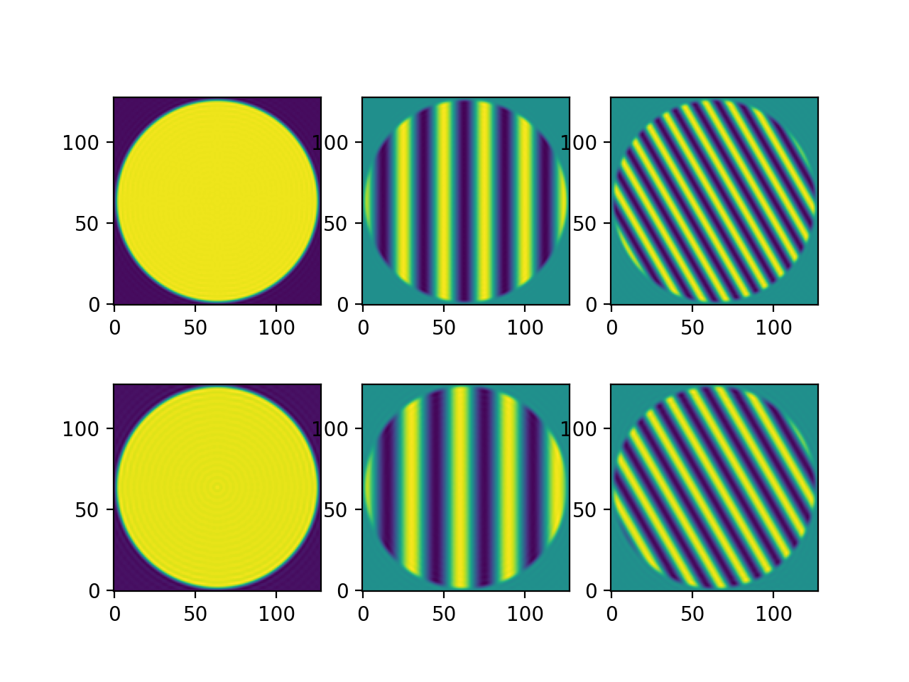
How does it look like? Let us apply a circular aperture to the field and plot it. The field is a cross section of a plane wave with wave vector defined by the wavelength, pixel size and direction (beta, phi) as can be seen in the images.

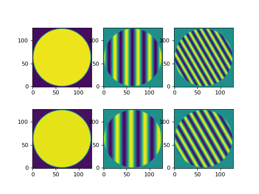
Fig. 5 The real part of the Ex component of the EM field for the three directions (beta, phi) and two wavelengths. Top row is for 500nm data, bottom row is 600nm data. (Source code, png, hires.png, pdf)¶

Field vector¶

For 1D and 2D simulations with a non-iterative algorithm we use field vector instead. There are conversion functions that you can use to build field data from field vector and vice-versa, e.g:

>>> fvec = dtmm.field.field2fvec(field)
>>> fvec.shape
(3, 2, 128, 128, 4)
>>> field = dtmm.field.fvec2field(fvec)
>>> field.shape
(3, 2, 4, 128, 128)