Introduction
dtmm is an electro-magnetic field transmission and reflection calculation engine and visualizer. It can be used for calculation of transmission or reflection properties of layered homogeneous or inhomogeneous materials, such as confined liquid-crystals with homogeneous or inhomogeneous director profile. DTMM stands for Diffractive Transfer Matrix Method and is an adapted Berreman 4x4 transfer matrix method and an adapted 2x2 extended Jones method. Details of the method are given in … some future paper.
Note
Although dtmm was mainly developed for 3D simulations, you can use the package for standard 4x4 calculation in 1D and in 2D.
See also
If you are into transmission optical microscopy simulations you may want to check nemaktis, which uses dtmm as one of the back-ends.
License
dtmm is released under MIT license so you can use it freely. Please cite the package if you use it to prepare plots for scientific paper. See the DOI badge in the repository
Contributors
I thank the following people for contributing and for valuable discussions:
Alex Vasile
Guilhem Poy
Highlights
Easy-to-use interface.
Fast and efficient code.
Support for the nematic director, Q tensor or dielectric tensor input data.
Computes transmission and reflection from the material.
Computes interference and diffraction effects.
Biaxial, uniaxial and isotropic material supported.
Fast iterative algorithm for 3D data - with tunable accuracy.
Non-iterative algorithm for 2D data - equivalent to the iterative algorithm with max accuracy settings.
Exact calculation for homogeneous layers (1D).
EM field visualizer (polarizing microscope simulator) allows you to simulate:
Light source intensity.
Polarizer/analyzer orientation and type (LCP, RCP or linear).
Phase retarders (lambda/4, lambda/2).
Sample rotation.
Focal plane adjustments.
Koehler illumination (field aperture).
Objective aperture.
Immersion or standard microscopes.
Cover glass aberration effects.
Color rendering (RGB camera simulations based on CIE color matching functions).
Pre-defined spectral response for monochrome CMOS cameras.
Status and limitations
dtmm was developed mainly for light propagation through liquid crystals, but it can also be used for simple 1D simulations using Jones calculus, or transfer matrix method. See the tutorial section for details. There are still some unresolved issues and limitations. These limitations are likely to be improved/implemented in the future (Contributions are welcome):
Limited color rendering functions and settings - no white balance correction of computed images.
Optimized for non-dispersive material. You have to split the calculation over different wavelengths and provide the optical data manually to simulate dispersive material.
Regular-spaced mesh only with equal spacing in x and y directions.
Note
EM field propagation calculation based on the iterative and non-iterative approach for 2D and 3D is exact for homogeneous layers, but it is approximate for inhomogeneous layers. It works good for slowly varying refractive index material (e.g. confined liquid crystals with slowly varying director field).
The package is still evolving, so there may be some small API changes in the future. Other than that, the package is fully operational. Play with the example below to get an impression on how it works.
Example
>>> import dtmm
>>> import numpy as np
>>> NLAYERS, HEIGHT, WIDTH = (60, 96, 96)
>>> WAVELENGTHS = np.linspace(380,780,9)
Build sample optical data:
>>> optical_data = dtmm.nematic_droplet_data((NLAYERS, HEIGHT, WIDTH),
...     radius = 30, profile = "r", no = 1.5, ne = 1.6, nhost = 1.5)
Build illumination data (input EM field):
>>> field_data_in = dtmm.illumination_data((HEIGHT, WIDTH), WAVELENGTHS,
...       pixelsize = 200)
Transmit the field through the sample:
>>> field_data_out = dtmm.transfer_field(field_data_in, optical_data)
Visualize the transmitted field with matplotlib plot:
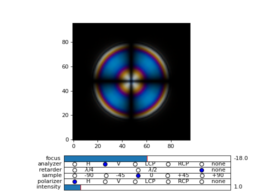
>>> viewer = dtmm.pom_viewer(field_data_out)
>>> viewer.set_parameters(sample = 0, polarizer = "h",
...      focus = -18, analyzer = "v")
>>> fig, ax = viewer.plot() #creates matplotlib figure and axes
>>> fig.show()

Fig. 1 Simulated optical polarizing microscope image of a nematic droplet with a radial nematic director profile (a point defect in the middle of the sphere). You can use sliders to change the focal plane, polarizer, sample rotation, analyzer, and light intensity. (Source code, png, hires.png, pdf)
Curious enough? Read the Quickstart Guide.
Contact
Andrej {dot} Petelin {at} gmail {dot} com