Tutorial
Jones calculus (1D)
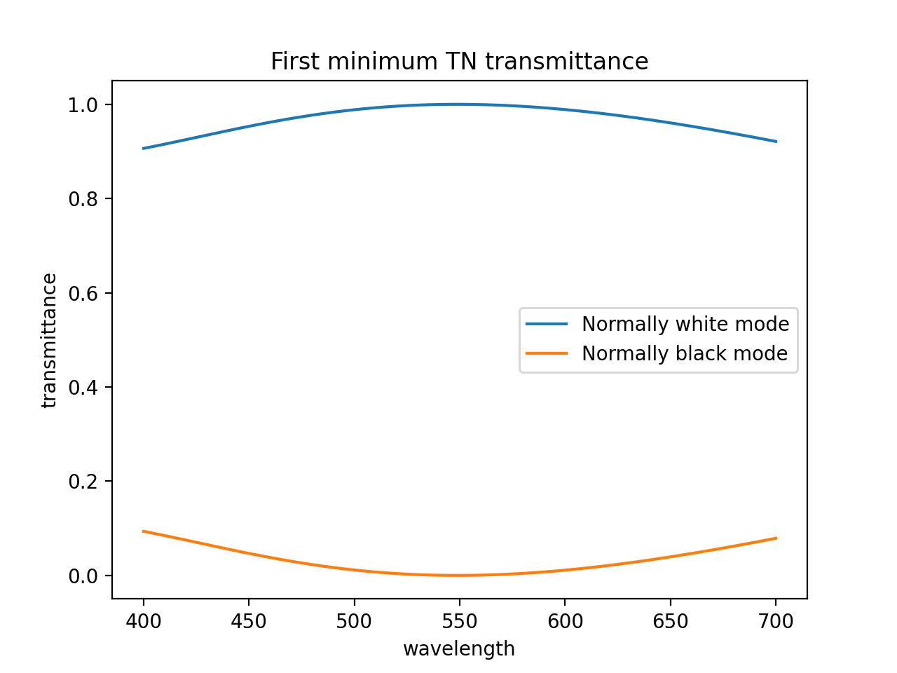
You can use the package for simple normal incidence Jones calculus. In the dtmm.jones you will find all the functionality to work with jones calculus. For example, we can compute the transmittance properties of a simple Twisted Nematic director profile. We compute wavelength-dependent transmittance of normally white and normally black TN modes. We build a left-handed twisted nematic in a 4 microns cell and in the first minimum condition - max transmission at 550 nm.
The matrix creation functions in the jones module obey numpy broadcasting rules, so we can build and multiply matrices at different wavelengths simultaneously. See the source code of the example below.
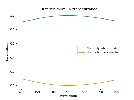
Fig. 6 (Source code, png, hires.png, pdf)
Transfer Matrix Method (1D)
For simulations in 1D you have several options using tmm. You can use the standard 4x4 transfer matrix approach, which allows you to study reflections from the surface, and there are several options for transmission calculations. In addition to 4x4, you can take the scattering matrix formulation (the 2x2) approach without reflections or with a single fresnel reflection. The 4x4 approach also allows you to perform single-reflection calculation (disabling interference effect) in case you have thicker samples. the details on the he 4x4 transfer matrix approach can be found tin the literature, e.g. Birefringent Thin Films and Polarizing Elements by McCall, Hodgkinson and Wu.
Run the source code and read the comments of the examples below to learn how to use the tools for 1D analysis using 4x4 approach.
Single layer reflection
In this example, we calculate reflections off a single 2 micron thick layer of material with refractive index of 1.5. See the source code for additional detail of the example below.
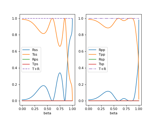
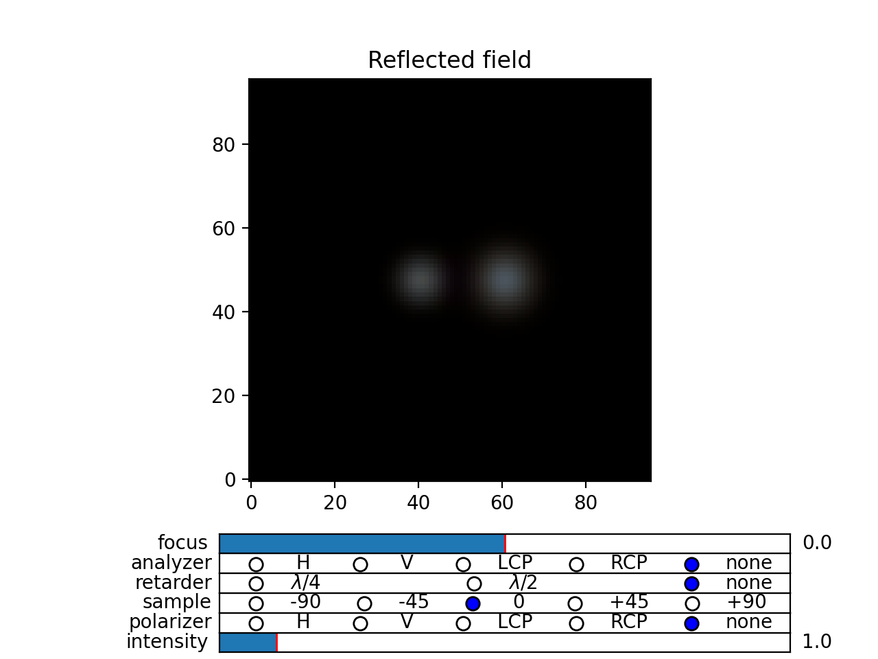
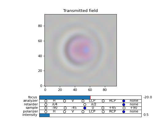
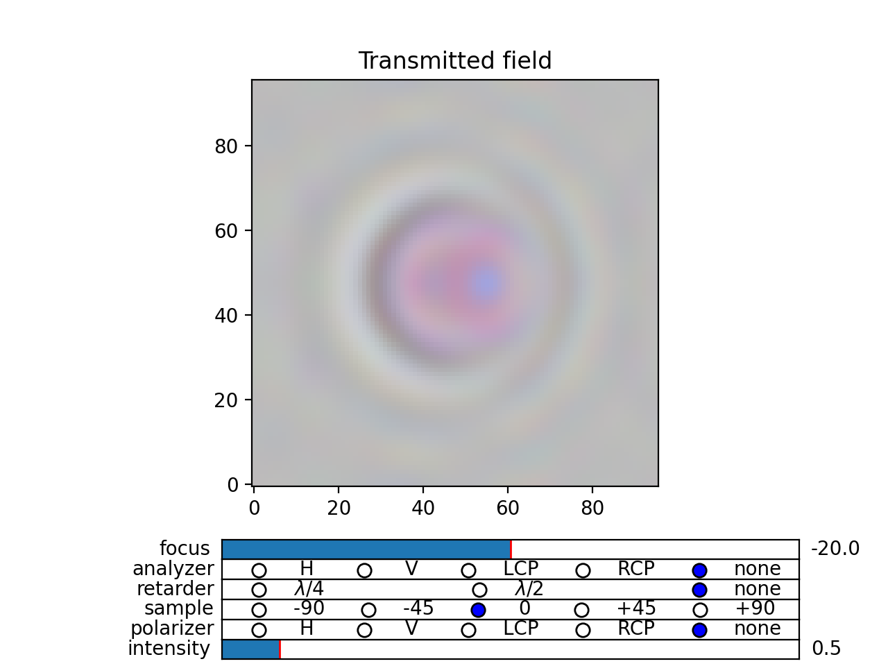
Fig. 7 Reflection and transmission properties of a single layer material. (Source code, png, hires.png, pdf)
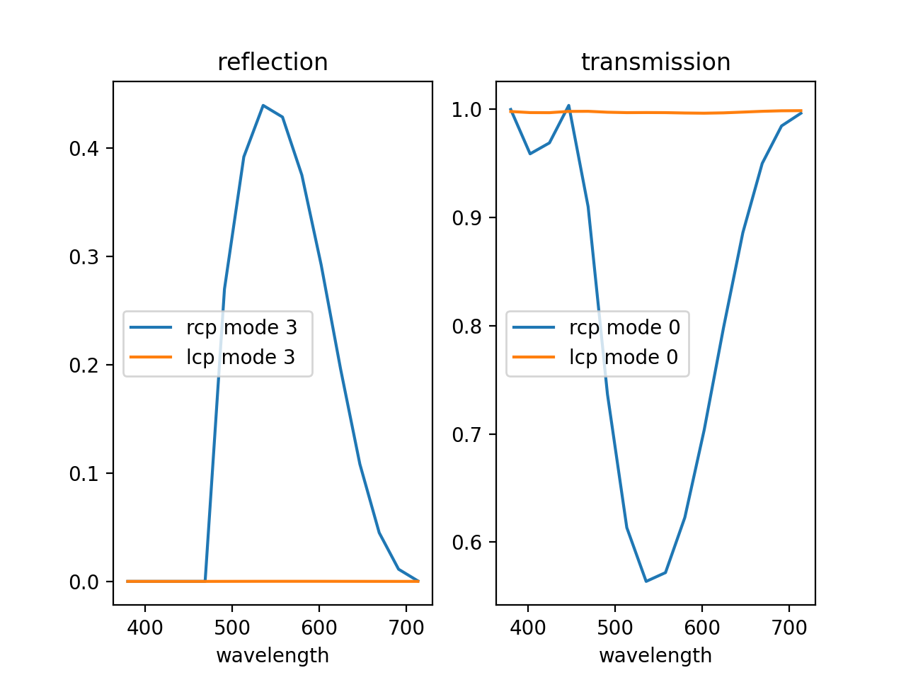
Cholesteric reflection
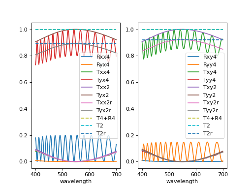
In this example we calculate reflections off a cholesteric material. See the source code for additional details of the example below.
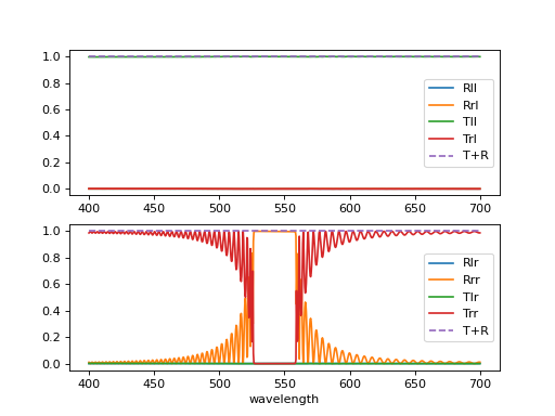
Fig. 8 Reflection and transmission properties of a cholesteric LC with a reflection band at 550 nm. (Source code, png, hires.png, pdf)
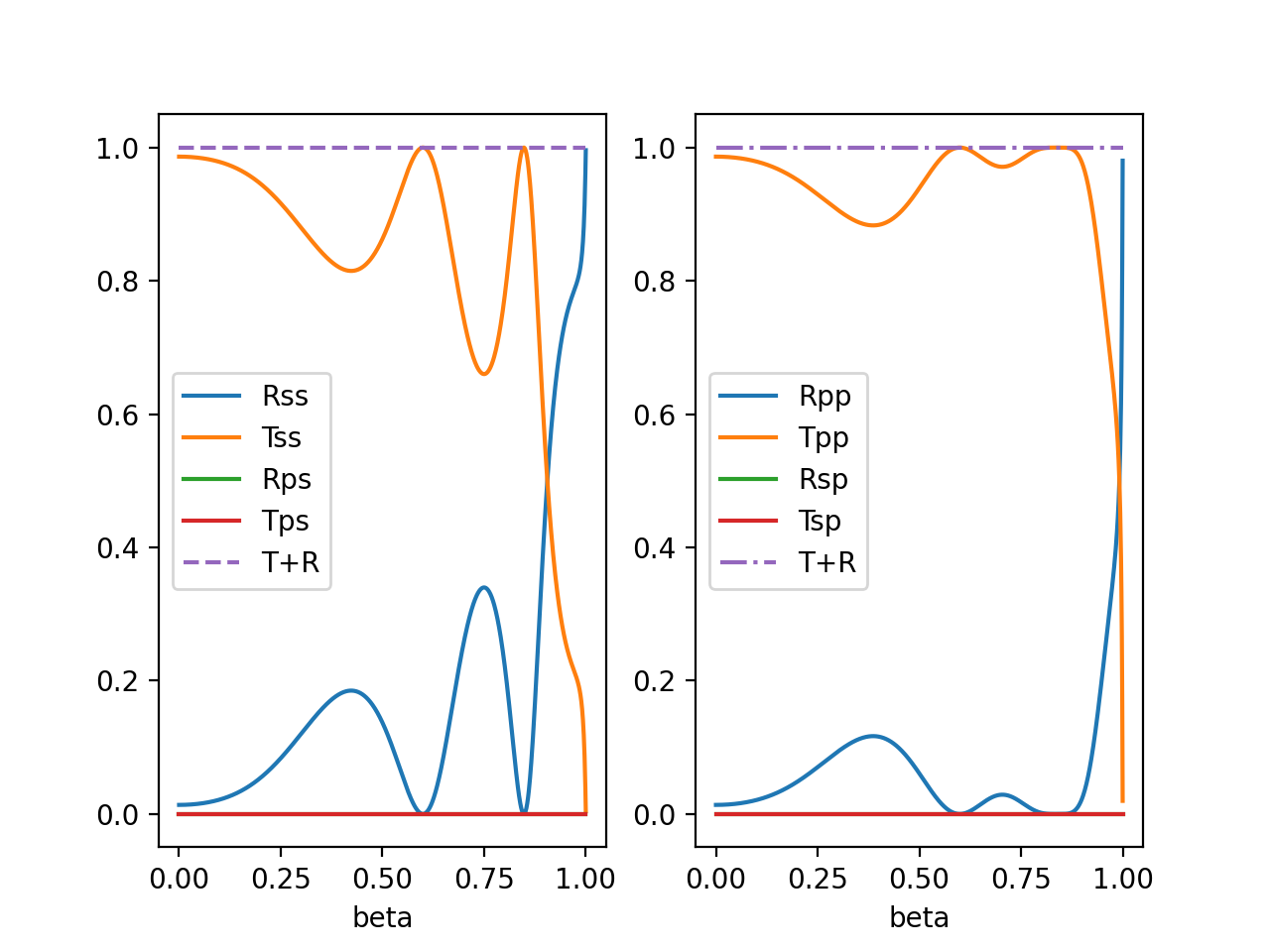
Twisted nematic transmission
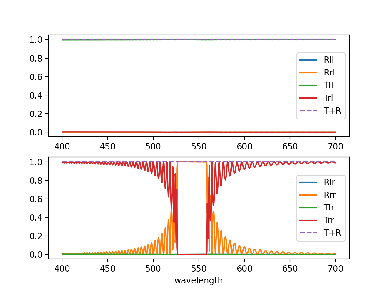
In this example we compute the transmittance through 90 degree twisted nematic configured in first minimum condition (4 micron cell, refractive index anisotropy of 0.12). Here we demonstrate and show differences between the 4x4 approach and two versions of 2x2 approach - with reflections and without.

Fig. 9 Reflection and transmission properties of a twisted nematic film (with film-to-air interfaces) (Source code, png, hires.png, pdf)
2D simulations
For 2D simulations, you can use the non-iterative 2D 4x4 approach developed in tmm2d. It works by writing the 4x4 matrices in Fourier space. At a given z position in space, and for a given computation box size and resolution, each wave can be described as a sum of N propagating modes. Therefore, for each of the inhomogeneous layers one writes a NxNx4x4 transfer matrix. Because of the NxN complexity, this approach works well for smaller sized computation cells involving only few modes. See the examples below for details.
Cholesteric reflection grating
In this example we calculate reflections from a tilted cholesteric sample, which produces a grating and mirror-like reflections. We plot optical microscope image formation and reflection efficiency for LCP and RCP input polarizations.

Fig. 10 (png, hires.png, pdf) (Source code)

Fig. 11 (png, hires.png, pdf) (Source code)

Fig. 12 (png, hires.png, pdf) (Source code)
3D simulations
In 3D, one may be tempted to develop the same non-iterative approach as for 2D. However, this becomes impractical because of the size of the matrices and computational complexity. Although you can find the implementation in tmm3d, this was developed for reference and testing, and it was not really meant to be useful in practice. Instead, for computations in 3D, we use an iterative algorithm. Instead of writing the transfer matrices and multiplying the matrices together to form a material characteristic matrix, one works with field vector in real space and transfers it through the layers in a split-step fashion. The layer is viewed as a thin inhomogeneous birefringent film and a thick homogeneous layer.
First, the field is transferred through the thin film in real space, acquiring phase change (with reflections), then the field is propagated by matrix multiplication if Fourier space. It is a bit more technical than that, and details of the non-iterative method is given in some future paper. Below you will find some technical information and examples of use.
Interference and reflections
By default, interference and reflections are neglected in the computation. You can enable interference by specifying how many passes to perform and using the 4x4 method
>>> field_out = dtmm.transfer_field(field_in, optical_data, npass = 5, method = "4x4")
or using the 2x2 method, assuming most reflections come from interlayer reflections and not from the inhomogeneities, in example, reflactions from the first air-sample interface and the last sample-air interface jou can do
>>> field_out = dtmm.transfer_field(field_in, optical_data, reflection = 1, npass = 3, method = "2x2")
If reflections come from the inhomogeneities you should call
>>> field_out = dtmm.transfer_field(field_in, optical_data, reflection = 2, npass = 3, method = "2x2")
Read further for details…
4x4 method
Dealing with interference can be tricky. The DTMM implements an adapted 4x4 transfer matrix method which includes interference, however, one needs to perform multiple passes (iterations) to compute the reflections from the material. With transfer matrix method one computes the output field (the forward propagating part and the backward propagating part) given the defined input field. In a typical experiment, the forward propagating part of the input field is known - this is the input illumination light. However, the backward propagating part of the input field is not know (the reflection from the surface of the material) and it must be determined.
The procedure to calculate reflections is as follows. First the method computes the output field by assuming zero reflections, so that the input field has no back propagating part. When light is transferred through the material, we compute both the forward and the backward propagating part of the output field. The back propagating part of the output field cancels all reflected waves from the material and the input light has no back propagating component of the field. To calculate reflections off the surface one needs to do it iteratively:
Initially input light is defined with zero reflections and transferred through the stack to obtain the output field.
After the first pass (first field transfer calculation), output light is modified so that the back propagating part of the field is completely removed. Then this modified light is transferred again through the stack in backward direction to obtain the modified input light which includes reflections.
After the second pass. Input light is modified to so that forward propagating part of the field matches the initial field, and the field is transferred through the stack again..
For low reflective material, three passes are usually enough to obtain a reasonable accurate reflection and transmission values. However, in highly reflective media (cholesterics) more passes are needed.
The calculation is done by setting the npass and norm arguments:
>>> field_data_out = dtmm.transfer_field(field_data_in, optical_data, npass = 3, norm = 2)
The npass argument defines number of passes (field transfers). You are advised to use odd number of passes when dealing with reflections. With odd passes you can inspect any residual back propagating field left in the output field, to make sure that the method has converged.
In highly reflective media, the solution may not converge. You must play with the norm argument, which defines how the output field is modified after each even pass.
with norm = 0 the back propagating part is simply removed, and the total intensity of the forward propagating part is rescaled to conserve total power flow. This method works well for weak reflections.
with norm = 1 the back propagating part is removed, and the amplitude of the fourier coefficients of the forward propagating part are modified so that power flow of each of the modes is conserved. This method work well in most cases, especially when reflections come from mostly the top and bottom surfaces.
with norm = 2, during each even step, a reference non-reflecting and non-interfering wave is transferred through the stack. This reference wave is then used to normalize the forward propagating part of the output field. Because of the additional reference wave calculation this procedure is slower, but it was found to work well in any material (even cholesterics).
2x2 method
The 2x2 method is a scattering method, it is stable (contrary to the 4x4 method) and it can also be used to compute interference. When npass>1, the method calculates fresnel reflections from the layers and stores intermediate results. As such, it is much more memory intensive as the 4x4 method (where intermediate results are not stored in memory). However, it is prone to greater numerical noise when dealing with highly reflecting media, such us cholesterics. Also, large number of passes are required for highly reflective media, so it can be used for weakly reflecting material only.
There are two reflection calculation modes. In the reflection = 1 mode, the field is Fourier transformed and mode coefficients are reflected from the interface between the effective layers (specified by the eff_data argument). If you want to calculate reflections from a stack of homogeneous layers, this gives an exact reflection calculation. For instance, to take into account reflections from the input and output interfaces, simply do
>>> field_out = dtmm.transfer_field(field_in, optical_data, reflection = 1, npass = 3, method = "2x2")
In the example above there will be no interlayer reflections in the sample, because the optical data is seen as an isotropic effective data with a mean refractive index when treating diffraction and reflection in light propagation. But, input and output layers have different refractive indices (n=1 by default), so you will see reflections from these interfaces.
In the reflection = 2 mode, the field is reflected from the inhomogeneous layers in real space. Consequently, this is not exact if the layers are homogeneous and the input light beam has a large number of off-axis waves, but it can be used when you want to see reflections from local structures. To take into account the dependence of off-axis wave reflection coefficient with the mode coefficient you must increase the diffraction quality, e.g.:
>>> field_out = dtmm.transfer_field(field_in, optical_data, diffraction = 5, reflection = 2, npass = 3, method = "2x2")
In the example above, reflections are cumulatively acquired from each of the interfaces in the optical data, including reflections from the input and output interfaces. If main reflections come from the input and output interfaces this will not be as accurate as reflection = 1 mode, but it will be more accurate if reflections are mainly due to the inhomogeneities in the optical data.
Examples
Surface reflections
In this example we calculate reflection and transmission of a spatially narrow light beam that passes a two micron thick isotropic layer of high refractive index of n = 4 at an angle of beta = 0.4. Already at three passes, the residual data is almost gone.
One clearly sees beam walking and multiple reflections and interference from both surfaces. See the examples/reflection_isolayer.py for details.

Fig. 13 (png, hires.png, pdf) Reflection and transmission of an off-axis (beta = 0.4) light beam from a single layer of two micron thick high refractive index material (n=4). Intensity is increased to a value of 100, to see the multiple reflected waves, (Source code)
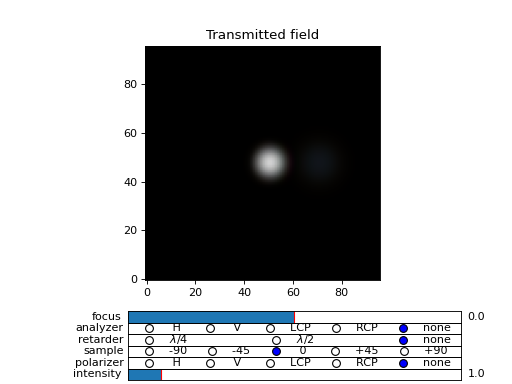
Fig. 14 (png, hires.png, pdf) Reflection and transmission of an off-axis (beta = 0.4) light beam from a single layer of two micron thick high refractive index material (n=4). Intensity is increased to a value of 100, to see the multiple reflected waves, (Source code)

Fig. 15 (png, hires.png, pdf) Reflection and transmission of an off-axis (beta = 0.4) light beam from a single layer of two micron thick high refractive index material (n=4). Intensity is increased to a value of 100, to see the multiple reflected waves, (Source code)
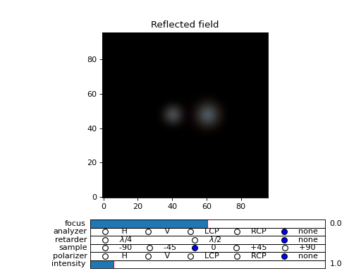
Fig. 16 (png, hires.png, pdf) Reflection and transmission of an off-axis (beta = 0.4) light beam from a single layer of two micron thick high refractive index material (n=4). Intensity is increased to a value of 100, to see the multiple reflected waves, (Source code)
Cholesterics
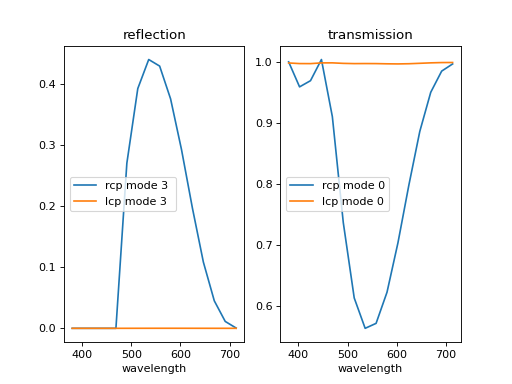
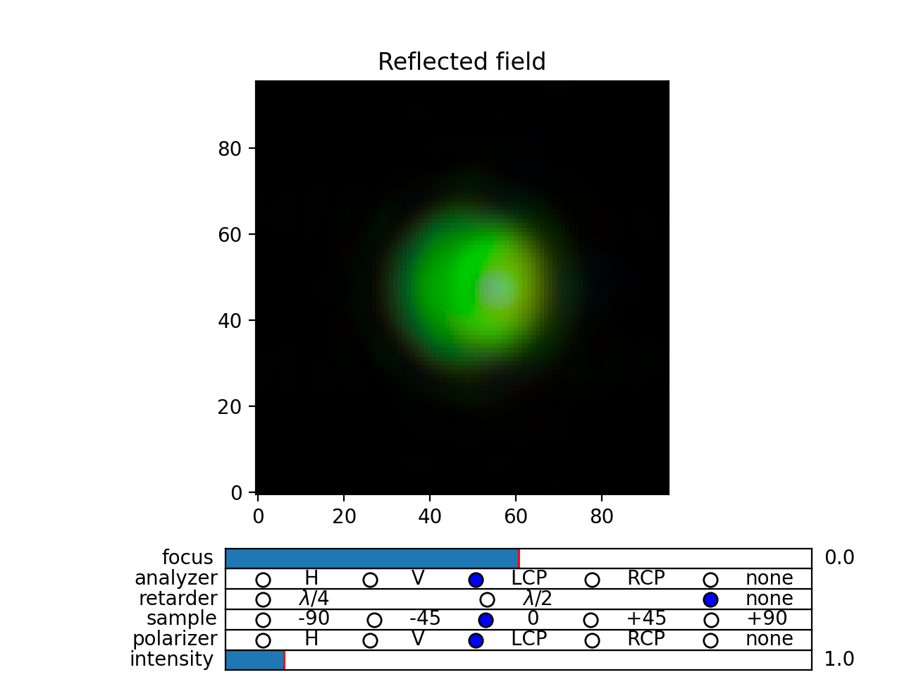
In this example, we use multiple passes to compute reflections of the cholesteric droplet. For cholesterics one should take the norm = 2 argument in the computation of the tranfered field.
The droplet is a left-handed cholesteric with pitch of 350 nm, which results in a strong reflection of right-handed light of wavelength 520 nm (350*1.5 nm). Already with npass = 5, the residual field has almost vanished.
In the example below, we simulated propagation of right-handed light with beta parameter beta = 0.2. See the examples/cholesteric_droplet.py for details.

Fig. 17 (png, hires.png, pdf) Reflection and transmission properties of a cholesterol droplet. (Source code)
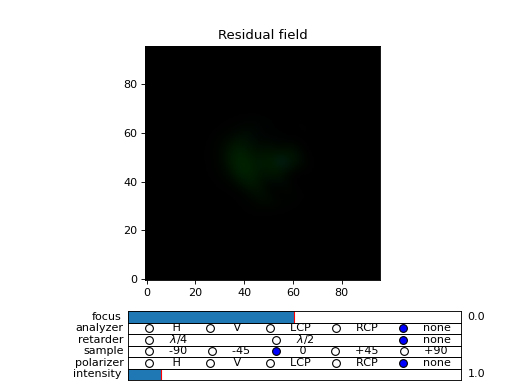
Fig. 18 (png, hires.png, pdf) Reflection and transmission properties of a cholesterol droplet. (Source code)
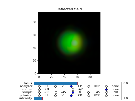
Fig. 19 (png, hires.png, pdf) Reflection and transmission properties of a cholesterol droplet. (Source code)
Standard TMM - no diffraction
You can use the dtmm package for 1D calculation. There are two options. Either you create a single pixel optical data that describes your 1D material and use the functions covered so far, or you do a standard Berreman or Jones calculation by computing the transfer matrices, and the reflectance and transmittance coefficients with functions found in dtmm.tmm. For coherent reflection calculation of complex 1D material this may be better/faster than using the dtmm.transfer.transfer_field(). Note that the diffractive method uses iterative algorithm to calculate coherent effects. With a standard 4x4 method in 1D case, these are done in a single step.
In the dtmm.tmm module you will find low-level implementation of the TMM method, and some high level function to simplify computations and use. Here we go through the high level API, while for some details on the implementation you should read the source code of the examples below.
Basics
Computation is performed in two steps. First we build a characteristic matrix of the stack, then we calculate transmitted (and reflected) field from a given field vector. Field vector now is a single 4-component vector. We will demonstrate the use on a 3D data that we were working on till now.
>>> d, epsv, epsa = dtmm.nematic_droplet_data((NLAYERS, HEIGHT, WIDTH),
...          radius = 30, profile = "x", no = 1.5, ne = 1.6, nhost = 1.5)
>>> f,w,p = dtmm.illumination_data((HEIGHT, WIDTH), WAVELENGTHS, diffraction = False,
...               pixelsize = PIXELSIZE, beta = 0., phi = 0.)
First we need to transpose the field data to field vector
>>> fin = dtmm.field.field2fvec(f)
Next we need to build phase constants (layer thickness times wavenumber)
>>> kd = [x*(dtmm.k0(WAVELENGTHS, PIXELSIZE))[...,None,None] for x in d]
Here we also added two axes for broadcasting. The epsv[i] and epsa[i] arrays are of shape
(HEIGHT, WIDTH, 3), we need to add two axes of len(1) to elements kd[i] because numpy broadcasting rules apply to arguments of the dtmm.tmm.stack_mat() that is used to compute the characteristic matrix. So now you do:
>>> cmat = dtmm.tmm.stack_mat(kd, epsv, epsa)
which computes layer matrices Mi and multiplies them together so that the output matrix is M = Mn…M2.M1. Then you call dtmm.tmm.transmit() to compute the tranmiiited and reflected fields (the reflected field is added to input field).
>>> fout = dtmm.tmm.transmit(fin,cmat)
That is it. You can now view this field with the field_viewer, but first you need to transpose it back to the original field data shape.
>>> field_data = dtmm.field.fvec2field(fout),w,p
>>> viewer = dtmm.field_viewer(field_data, diffraction = False)
Note the use of diffraction= False option which tells the field viewer that computed data is not diffraction-limited (and has not been calculated with the transfer_field dfunction and diffraction>0 argument). This way, data is displayed as is, without any plane-wave decomposition and filtering (by cutting non-propagating high frequency modes).
The stack_mat() takes an optional parameter method which can take a string value of “4x4”, “2x2” or “4x2”. The “4x4” is for standard Berreman - interference enabled calculation, The “4x2” method is for a 4x4 method, but with interference disabled by setting the phase matrix element to zeros for back propagating waves. This method is equivalent to method = “2x2” and reflection = 2 arguments in the dtmm.transfer.transfer_field(). The “2x2” method is for jones calculation. This method is equivalent to method = “2x2” and reflection = 0 arguments in the dtmm.transfer.transfer_field().
Nematic droplet example
See the source code of the examples to see additional details.
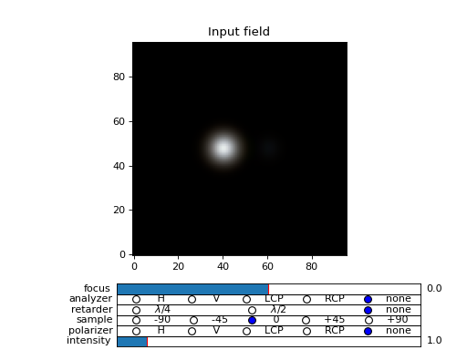
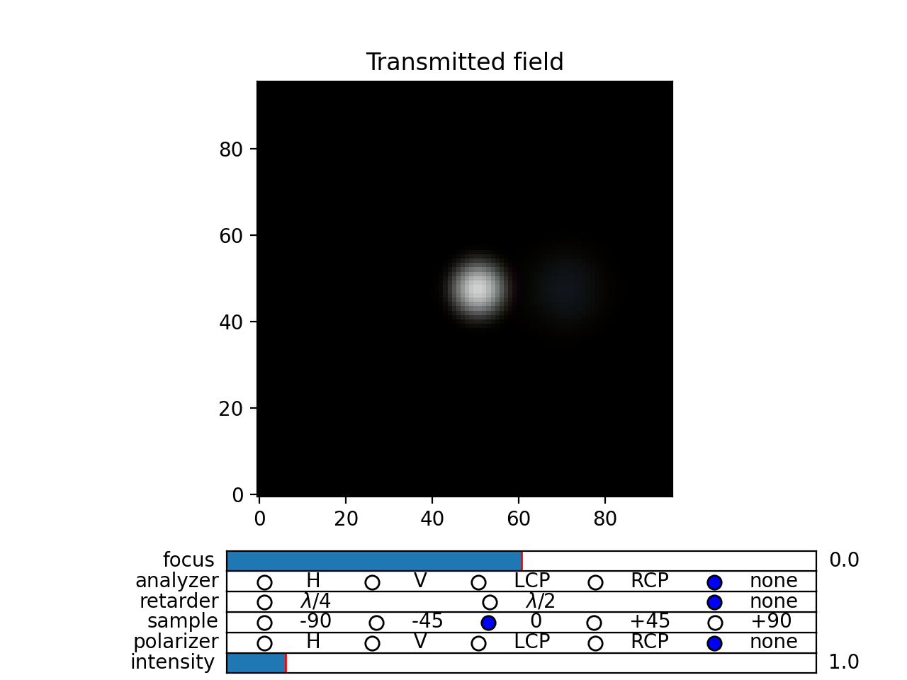
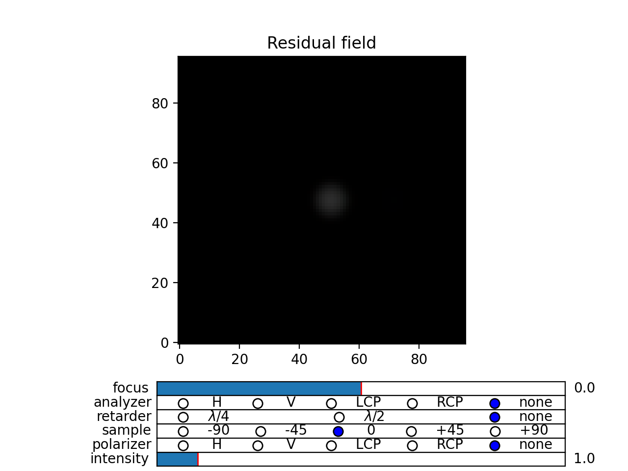
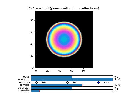
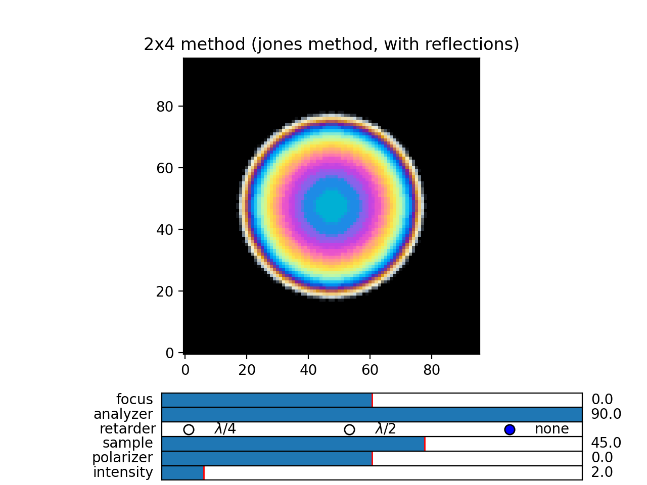
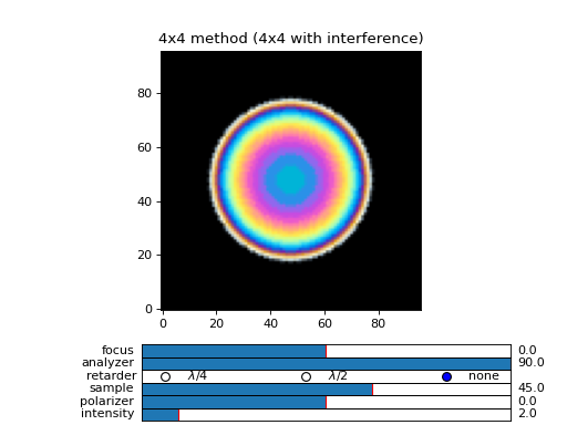
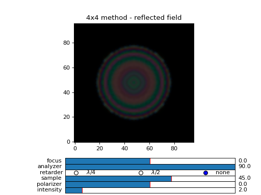
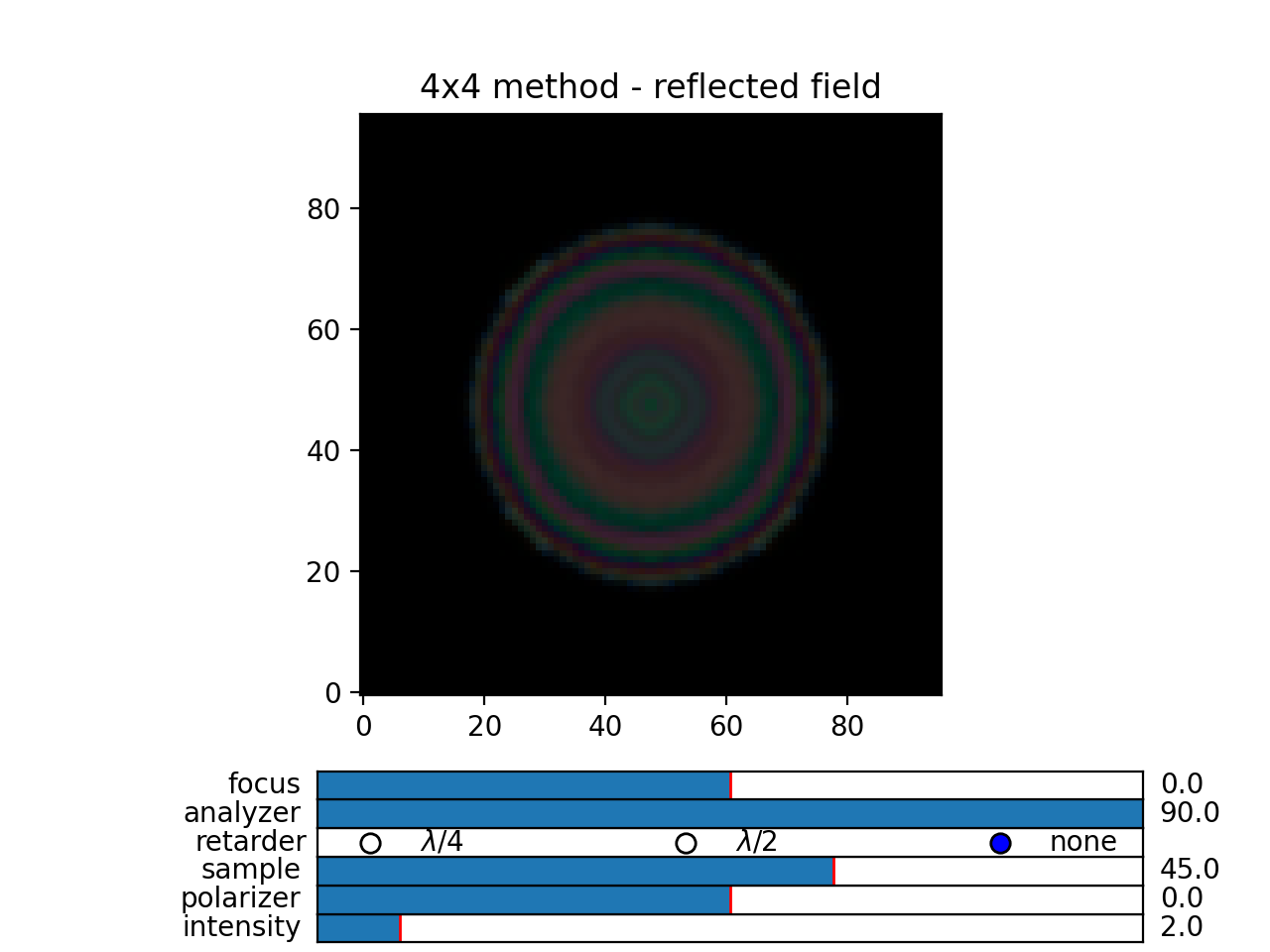
An example of a nematic droplet with planar director orientation, computed using 4x4 method with interference, 4x4 method without interference (single reflection) and 2x2 method with no reflections at all. All of these examples could be computed with transfer_field functions and diffraction = False argument… and the results of both methods should be identical (up to numerical precision).

Fig. 20 (png, hires.png, pdf) An example of extended jones calculation, berreman 4x4 with interference and with interference disabled methods to compute transmission of a white light through the nematic droplet with a planar director alignment, viewed between crossed polarizers. (Source code)

Fig. 21 (png, hires.png, pdf) An example of extended jones calculation, berreman 4x4 with interference and with interference disabled methods to compute transmission of a white light through the nematic droplet with a planar director alignment, viewed between crossed polarizers. (Source code)

Fig. 22 (png, hires.png, pdf) An example of extended jones calculation, berreman 4x4 with interference and with interference disabled methods to compute transmission of a white light through the nematic droplet with a planar director alignment, viewed between crossed polarizers. (Source code)

Fig. 23 (png, hires.png, pdf) An example of extended jones calculation, berreman 4x4 with interference and with interference disabled methods to compute transmission of a white light through the nematic droplet with a planar director alignment, viewed between crossed polarizers. (Source code)

Fig. 24 (png, hires.png, pdf) An example of extended jones calculation, berreman 4x4 with interference and with interference disabled methods to compute transmission of a white light through the nematic droplet with a planar director alignment, viewed between crossed polarizers. (Source code)
Field viewer
In addition to the Polarizing Optical Microscope viewer which was covered in the quick start guide, there is also a FieldViewer. The difference between the FieldViewer and POMViewer is that the latter works with 2x2 matrices, whereas FieldViewer works with 4x4 matrices.
Here we will cover some additional configuration options for the FieldViewer. The field viewer can be used to inspect the output field, or to inspect the bulk field data.
Projection mode
One powerful feature of the FieldViewer is the ability to project the waves and isolate the forward or backward propagating waves. This is how the images of the examples above were created, so to take the transmitted part of the field do:
>>> viewer = dtmm.field_viewer(field_data_out, mode = "t") #the transmitted part
to view the reflected part of the field do:
>>> viewer = dtmm.field_viewer(field_data_out, mode = "r") #the reflected part
When field viewer is called without the mode argument it performs no projection calculation. A power flow is calculated directly from the electro-magnetic field (Poynting vector times layer normal). As such, the power flow can be positive or negative. A negative power flow comes from the back propagating waves and it has to be stressed that negative values are clipped in the conversion to RGB. Therefore, when dealing with reflections and interference calculations, you should be explicit about the projection mode.
The numerical aperture
Another parameter that you can use is the betamax parameter. Some explanation on this is below, but in short, with betamax parameter defined in the field_viewer function you can simulate the finite numerical aperture of the objective. So to simulate an image taken by a microscope with NA of 0.4 do:
>>> viewer = dtmm.field_viewer(field_data_out, mode = "t", betamax = 0.4)
And if you want to observe ideal microscope lens image formation, set betamax to the value of refractive index). For instance an oil-immersion objective with n = 1.5 and NA 1.3 do
>>> viewer = dtmm.field_viewer(field_data_out, mode = "t", betamax = 1.3, n = 1.5)
but of course, here it is up to the user to calculate the output field for the output refractive index of 1.5.
Viewing bulk data
The field_viewer function can also be used to show bulk EM data in color. Here you will generally use it as
>>> viewer = dtmm.field_viewer(field_bulk_data, bulk_data = True)
Now the “focus” parameter has a role of selecting a layer index and the viewer shows the power of the EM field in the specified layer.
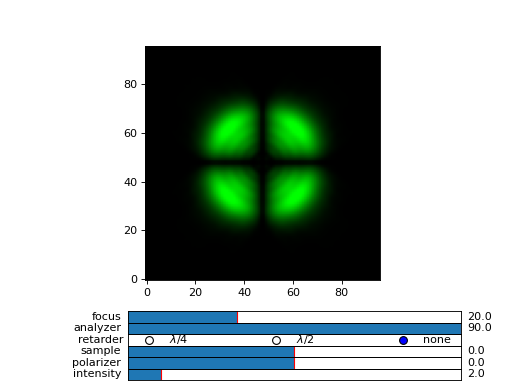
Fig. 25 Bulk viewer - viewing field in a specified layer. (Source code, png, hires.png, pdf)
The refractive index n, and betamax parameters are meaningless when using the field_viewer to visualize bulk data, except if you define a transmission or reflection mode. In this case, the viewer project the EM field and calculates the forward or backward propagating parts and removes the waves with beta value larger than the specified betamax parameter before calculating the intensity.
POM viewer
The Polarizing Optical Microscope viewer was covered in the quick start guite. The difference between the FieldViewer and POMViewer is that the latter works with 2x2 matrices, whereas FieldViewer works with 4x4 matrices. Internally, the POMViewer converts the field data to E-field (or jones field data):
>>> jones = dtmm.field.field2jones(f,dtmm.k0(WAVELENGTHS, PIXELSIZE))
This is done automatically when you call the:
>>> pom = dtmm.pom_viewer(field_data)
See the quick start quite for usage details.
Calculation accuracy
Effective medium
The algorithm uses a split-step approach where the diffraction calculation step is performed assuming a homogeneous effective medium. What this means is that if the input optical data consists of homogeneous layers, the algorithm is capable of computing the exact solution. However, the accuracy of the calculated results will depend on how well you are able to describe the effective medium of the optical stack. By default, isotropic medium is assumed, that is, for each layer in the stack an isotropic layer is defined and calculated from the input optical data parameters. You can also explicitly define the medium as:
>>> out = dtmm.transfer_field(field, data, eff_data = "isotropic")
If the layer cannot be treated as an isotropic layer on average, you should tell dtmm to use anisotropic layers instead, e.g.:
>>> out = dtmm.transfer_field(field, data, eff_data = "uniaxial")
or
>>> out = dtmm.transfer_field(field, data, eff_data = "biaxial")
Note
The ‘biaxial’ option is considered experimental. In the calculation of the diffraction matrix for biaxial medium the algorithm may not be able to properly sort the eigenvectors for beta values above the critical beta (for waveguiding modes). These modes are filtered out later in the process and controlled by the betamax parameter, so in principle, mode sorting is irrelevant for propagating modes. Consequently, you may see some warnings on mode sorting, but this should not affect the end results. This issue will be fixed at some point.
Internally, when specifying eff_data argument, the algorithm performs calculation of the effective medium with
>>> eff_data = dtmm.data.eff_data(data, "uniaxial")
which computes the spatially-varying dielectric tensor for each of the layers, performs averaging, and then converts the averaged tensor to eigenframe and converts it to the desired symmetry. You can use the above function to prepare effective layers and pass the computed result to
>>> out = dtmm.transfer_field(field, data, eff_data = eff_data)
For even higher accuracy, in more non-uniform systems where the mean dielectric tensor varies considerably across the layers you should define the effective medium for each of the layers separately:
>>> n_layers = len(data[0])
>>> eff_data = dtmm.data.eff_data(data, ("uniaxial",)*n_layers)
which performs averaging of the dielectric tensor only across the individual layer and defines a unique effective data for each of the layers. You can also do:
>>> out = dtmm.transfer_field(field, data, eff_data = ("uniaxial",)*n_layers)
You can also mix the symmetry e.g.
>>> eff_data = ("uniaxial","isotropic","biaxial",...) #length must match the number of layers
Please note that having different effective layers in the system significantly slows down the computation because the diffraction matrices need to be calculated for each of the layers, whereas if
>>> eff_data = "uniaxial"
the calculation of the diffraction matrix is done only once.
Note
You can set the default medium in the configuration file. See Configuration & Tips for details.
Diffraction quality
Diffraction calculation can be performed with different levels of accuracy. By default, diffraction and transmission through the inhomogeneous layer is calculated with a single step, assuming the field is a beam of light with a well defined wave vector. If your sample induces waves with higher frequencies, you should split the field into a sum of beams by defining how many beams to use in the diffraction calculation. For instance,
>>> out = dtmm.transfer_field(field, data, diffraction = 3)
in the diffraction calculation step, the method takes beams defined with beta parameters in a 3x3 grid of beta_x beta_y values defined between -betamax and +betamax, so a total of 9 beams (instead of a single beam when diffraction = 1). Therefore this will take significantly longer to compute. You can use any sensible integer value - this depends on the pixel size and domain size. For calculation of 100x100 grid with pixelsize of 50 nm and 500nm wavelength, the maximum sensible value is 100*50/500=10, but generally, above say diffraction = 7 you will not notice much improvement, but this depends on the material of course. In the extreme case, the most accurate calculation can be done by specifying
>>> out = dtmm.transfer_field(field, data, diffraction = np.inf)
or with a value of
>>> out = dtmm.transfer_field(field, data, diffraction = -1)
This triggers a full treatment of diffraction, transfers all waves within the beta < betamax. This method is very slow, and should not be used generally, except for very small samples.
Try experimenting yourself. As a rule of thumb, diffraction = 1 gives a reasonable first approximation and is very fast to compute, and with diffraction = 5 you are very close to the real thing, but about 5*5 slower to compute.
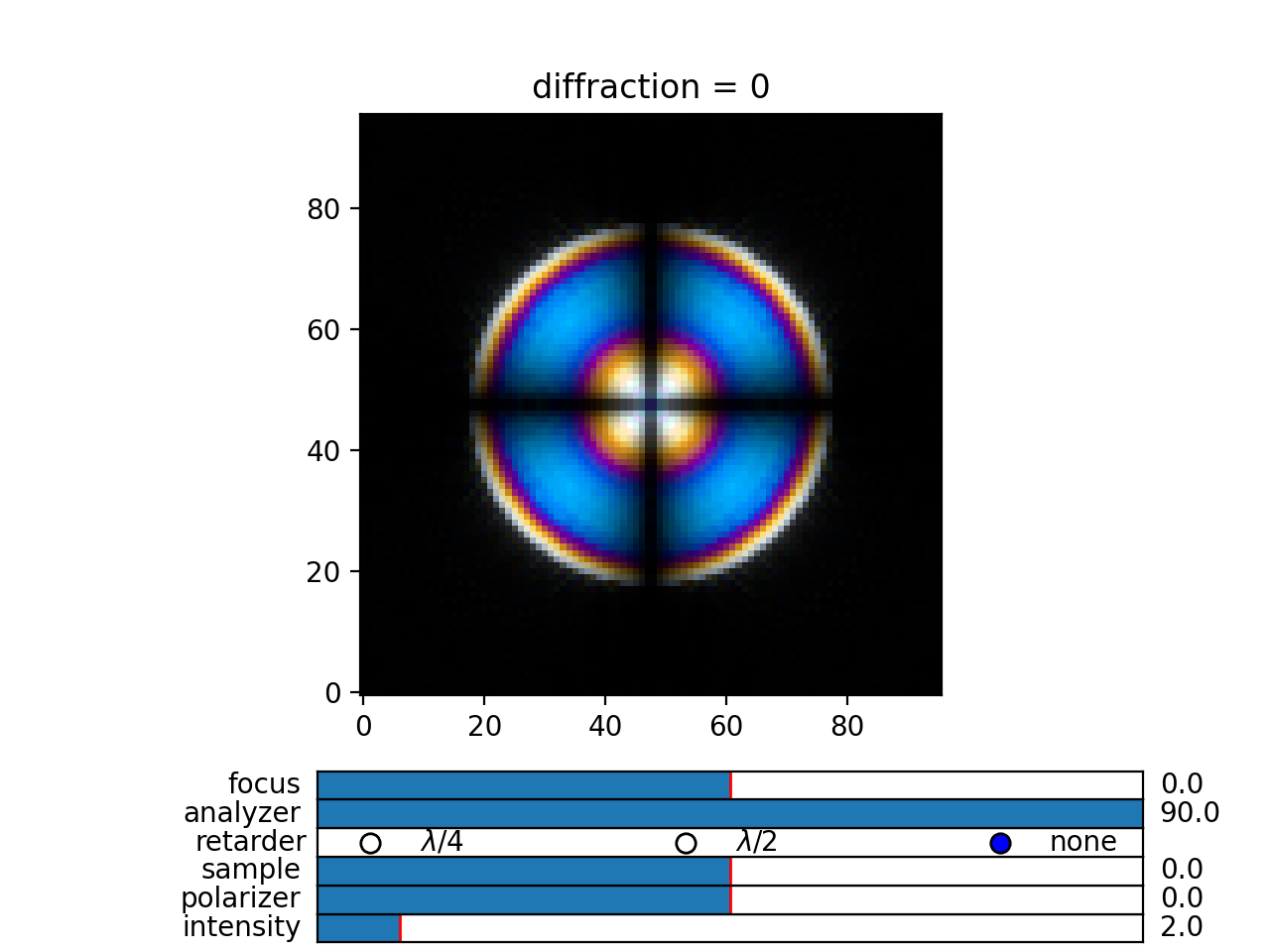
In the examples below we show difference between several diffraction arguments (0,1,5). With diffraction = 0, the method does not include diffraction effects. With diffraction = 1 and 5, one can see that due to diffraction a halo ring appears and the appearance of colors is slightly different for all three methods.

Fig. 26 (png, hires.png, pdf) A comparison of diffraction = 0, diffraction = 1, and diffraction = 5 transmission calculations of same radial nematic droplet. See source for details on optical parameters. (Source code)
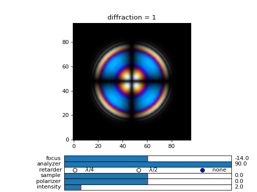
Fig. 27 (png, hires.png, pdf) A comparison of diffraction = 0, diffraction = 1, and diffraction = 5 transmission calculations of same radial nematic droplet. See source for details on optical parameters. (Source code)
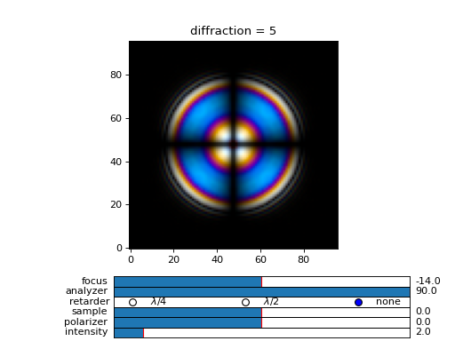
Fig. 28 (png, hires.png, pdf) A comparison of diffraction = 0, diffraction = 1, and diffraction = 5 transmission calculations of same radial nematic droplet. See source for details on optical parameters. (Source code)
Note
You can also disable diffraction calculation step by setting the diffraction = False to trigger a standard 2x2 jones calculation or 4x4 Berreman calculation (when method = 4x4)
On the betamax parameter
The betamax parameter defines the maximum value of the plane wave beta parameter in the diffraction step of the calculation. When decomposing the field in plane waves, the plane wave with the beta parameter higher than the specified betamax parameter is neglected. In air, the maximum value of beta is 1. A plane wave with beta = 1 is a plane wave traveling in the lateral direction (at 90 degree with respect to the layer normal). If beta is greater than 1 in air, the plane wave is no longer a traveling wave, but it becomes an evanescent wave and the propagation becomes unstable in the 4x4 method (when method = “4x4” is used in the computation). In a medium with higher refractive index, the maximum value for a traveling wave is the refractive index beta=n. Generally you should use betamax < n, where n is the lowest refractive index in the optical stack (including the input and output isotropic layers). Therefore, if you should set betamax < 1 when the input and output layers are air with n=1. Some examples:
>>> out = dtmm.transfer_field(field, data, betamax = 0.99, method = '4x4') #safe
>>> out = dtmm.transfer_field(field, data, betamax = 1,  method = '4x4') #unsafe
>>> out = dtmm.transfer_field(field, data, betamax = 1.49,  method = '4x4', nin = 1.5, nout = 1.5) #safe
>>> out = dtmm.transfer_field(field, data, betamax = 1.6, method = '4x4', nin = 1.5, nout = 1.5) #unsafe
When dealing only with forward waves (the 2x2 approach).. the method is stable, and all above examples are safe to execute:
>>> out = dtmm.transfer_field(field, data, betamax = 2, method = '2x2') #safe
However, there is one caveat.. when increasing the diffraction accuracy it is also better to stay in the betamax < 1 range to increase computation speed. For instance, both examples below will give similarly accurate results, but computation complexity is higher when we use higher number of waves in the diffraction calculation step:
>>> out = dtmm.transfer_field(field, data, betamax = 2, diffraction = 5) #safe but slow
>>> out = dtmm.transfer_field(field, data, betamax = 1, diffraction = 3) #safe and faster
Color Conversion
In this tutorial you will learn how to transform specter to RGB colors using CIE 1931 standard observer color matching function (see CIE 1931 wiki pages for details on XYZ color space). You will learn how to use custom light source specter data and how to compare the simulated data with experiments (images obtained by a color camera). First we will go through some basics, but you can skip this part and go directly to Color cameras
Background
In the dtmm.color there is a limited set of functions for converting computed specters to RGB images. It is not a full color engine, so only a few color conversion functions are implemented. The specter is converted to color using a CIE 1931 color matching function (CMF). Conversion to color is performed as follows. Specter data is first converted to XYZ color space using the CIE 1931 standard observer (5 nm tabulated) color matching function data. Then the image is converted to RGB color space (using a D65 reference white point) as specified in the sRGB standard (see sRGB wiki pages for details on sRGB color space). Data values are then clipped to (0.,1.) and finally, sRGB gamma transfer function is applied.
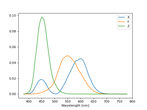
CIE 1931 standard observer
CIE 1931 color matching function can be loaded from table with.
>>> import dtmm.color as dc
>>> import numpy as np
>>> cmf = dc.load_cmf()
>>> cmf.shape
(81, 3)
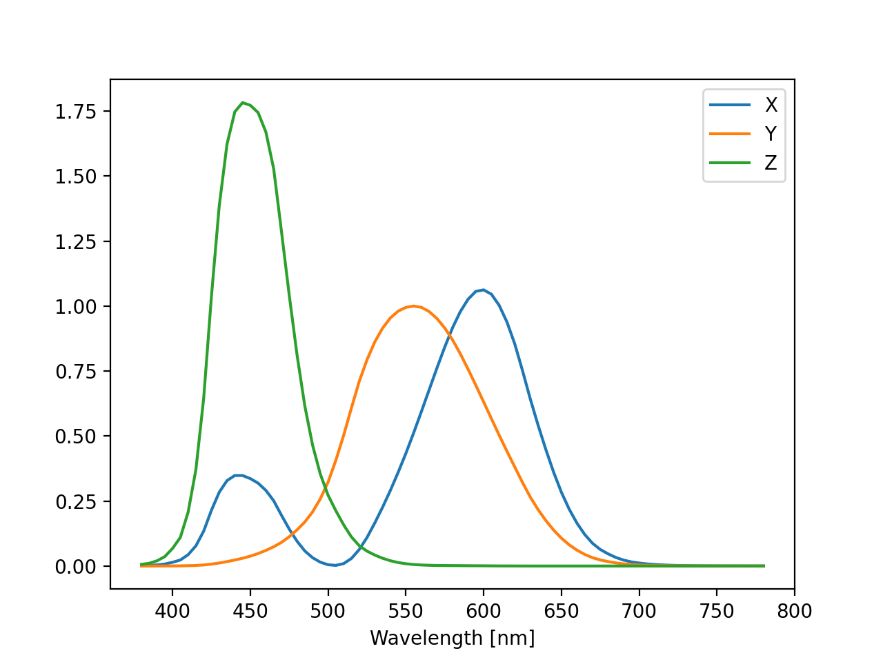
It is a 5nm tabulated data (between 380 and 780 nm) of 2-deg XYZ tristimulus values - a numerical representation of human vision system with three cones. This table is used to convert specter data to XYZ color space.
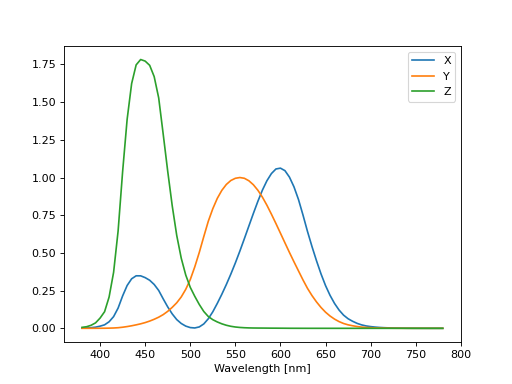
Fig. 29 XYZ tristimulus values. (Source code, png, hires.png, pdf)
D65 standard illuminant
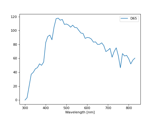
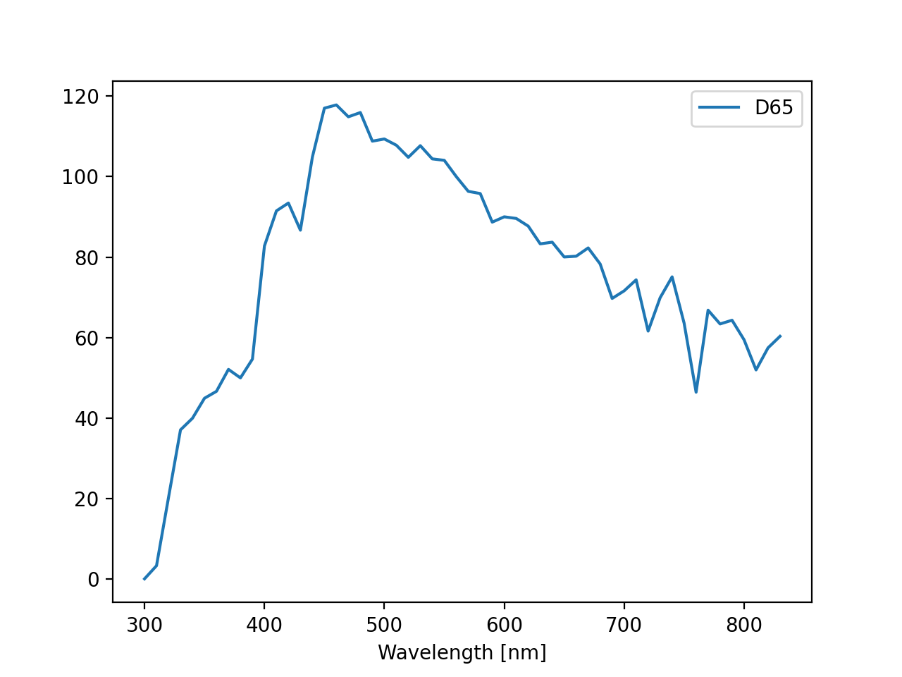
CIE also defines several standard illuminants. We will work with a D65 standard illuminant, which represents natural daylight. Its XYZ tristimulus value is used as a reference white color in the sRGB standard.
>>> spec = dc.load_specter()

Fig. 30 D65 color specter from 5nm tabulated data. (Source code, png, hires.png, pdf)
XYZ Color Space
The CMF table and D65 specter are defined so that resulting RGB image gives a white color. To convert specter to XYZ color space the specter dimensions has to match CMF table dimensions. CIE 1931 CMF is defined between 380 and 780 nm, while the D65 specter is defined between 300 and 830 nm. Let us match the specter to CMF by interpolating D65 tabulated data at CMF wavelengths:
>>> wavelengths, cmf = dc.load_cmf(retx = True)
>>> spec = dc.load_specter(wavelengths)
Now we can convert the specter to XYZ value with:
>>> dc.spec2xyz(spec,cmf)
array([2008.69027494, 2113.45495097, 2301.13095117])
Typically you will want to work with a normalized specter:
>>> spec = dc.normalize_specter(spec,cmf)
>>> xyz = dc.spec2xyz(spec,cmf)
>>> xyz
array([0.95042966, 1.        , 1.08880057])
Here we have normalized the specter so that the resulting XYZ value has the Y component equal to 1 (full brightness).
SRGB Color Space
Resulting XYZ can be converted to sRGB (using sRGB color primaries) with
>>> linear_rgb = dc.xyz2srgb(xyz)
>>> linear_rgb
array([0.99988402, 1.00003784, 0.99996664])
Because we have used a D65 specter data to compute the XYZ tristimulus values, the resulting RGB equals full brightness white color [1,1,1] (small deviation comes from the numerical precision of the XYZ2RGB color matrix transform). Note that Color matrices in the standard are defined for 8bit transformation. When converting float values to unsigned integer (8bit mode), these values have to be multiplied with 255 and clipped to a range of [0,255]. Finally, we have to apply sRGB gamma curve to have this linear data ready to display on a sRGB monitor.
>>> rgb = dc.apply_srgb_gamma(linear_rgb)
Since conversion to sRGB color space (from the input specter values) is a standard operation, there is a helper function to perform this transformation in a single call:
>>> rgb2 = dc.specter2color(spec,cmf)
>>> np.allclose(rgb,rgb2)
True
Transmission CMF
We can define a transmission color matching function. The idea is to have the CMF function defined for a transmission coefficients for a specific illumination so that the transmission computation becomes independent on the actual light spectra used in the experiment. For example, say we have computed transmission coefficients for a given set of wavelengths
>>> wavelengths = [380,480,580,680,780]
>>> coefficients = [1,1,1,1,1]
We would like to construct a color matching function that will convert these coefficient to color, assuming a given light spectrum. We can build a transmission color matching function with
>>> tcmf = dc.cmf2tcmf(cmf, spec)
or we could have loaded this directly with:
>>> tcmf2 = dc.load_tcmf()
>>> np.allclose(tcmf,tcmf2)
True

Fig. 31 D65-normalized XYZ tristimulus values. (Source code, png, hires.png, pdf)
this way we defined a new CMF function that converts unity transmission curve to bright white color (We are using D65 illuminant here).
>>> rgb3 = dc.specter2color([1]*81,tcmf)
>>> import numpy as np
>>> np.allclose(rgb,rgb3)
True
All fair, but we would not like to compute transmission coefficients at all 81 wavelengths defined in the original CMF data. We need to integrate the CMF function
>>> itcmf = dc.integrate_data(wavelengths, np.linspace(380,780,81), tcmf)
which results in a new CMF function applicable to transmission coefficients defined at new (different) wavelengths
We could have built this data directly by:
>>> itcmf = dc.load_tcmf(wavelengths)
Now we can compute
>>> rgb4 = dc.specter2color(coefficients,itcmf)
>>> import numpy as np
>>> np.allclose(rgb,rgb4)
True
Color Rendering
Not all colors can be displayed on a sRGB monitor. Colors that are out of gamut (R,G,B) chanels are larger than 1. or smaller than 0. are clipped. For instance, a D65 light that gives (R,G,B) = (1,1,1)* intensity filtered with a 150 nm band-pass filter already has colors clipped at some higher values of intensities. These colors are more vivid and saturated at light intensity of 1.
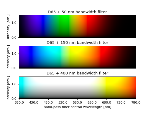
Fig. 32 An example of color rendering of a D65 illuminant filtered with a band-pass filter. If the illuminant is too bright, color clipping may occur. (Source code, png, hires.png, pdf)
Also, with sRGB color space we cannot render all colors, especially in the green part of the spectrum. For example, let us compute RGB values of a D65 light filtered with a band-pass filter between 500 and 550 nm.
>>> tcmf = dc.load_tcmf([500,550])
>>> xyz = dc.spec2xyz([1.,1.], tcmf)
>>> rgb = dc.xyz2srgb(xyz)
>>> rgb
array([-0.37267476,  0.67704885, -0.0234957 ])
gives a strong negative value in the red channel, which shows that the color is too saturated to be displayed in a sRGB color space. After we apply gamma (which clips the RGB channels to (0,1.)) we get
>>> dc.apply_srgb_gamma(rgb)
array([0.        , 0.84176254, 0.        ])
with the blue and red channel clipped. We should have used wide-gamut color space and a monitor capable of displaying wider gamuts to display this color properly. As stated already, this package was not intended to be a full color management system and you should use your own CMS system if you need more complex color transforms and rendering.
Color cameras
By default, in simulations light source is assumed to be the D65 illuminant. The reason is that with a D65 light source the color of fully transmissive filter is neutral gray (or white) when using the CIE color matching functions. If you want co compare with experiments, when using D65 light in simulation, you should do a proper white balance correction in your camera to obtain similar color rendering of the images obtained in experiments.
Another option is to match the illuminant used in simulation to the illuminant used in experiments. Say you have an illuminant data stored in a file called “illuminant.dat”, you can create a cmf function by
>>> cmf = dc.load_tcmf(wavelengths, illuminant = "illuminant.dat")
Afterwards, it is possible to set this illuminant in the field_viewer or pom_viewer.
>>> viewer = dtmm.pom_viewer(field_data, cmf = cmf)
For a standard A illuminant the example from the front page look like this:
Fig. 33 A hello world example, but this time, illumination was performed with a standard A illuminant. (Source code, png, hires.png, pdf)
Now, to compare this with the experimentally obtained images, you should disable all white balance correction in your camera, or if your camera has this option, set the white balance to day-light conditions. This way your color camera will transform the image assuming a D65 light source illuminant, just as the dtmm package does when it computes the RGB image. Also, non-scientific SLR cameras typically use some standard color profile that tend to increase the saturation of colors. Probably it is best to use a neutral or faithful color profile if your camera provides you with this option.
Monochrome cameras
To simulate a monochrome camera, you also have to construct a proper color matching function. For example, for a standard CMOS camera, to build a tcmf function for light source approximated with three wavelengths and an illuminant specified by the illuminant table, do:
>>> wavelengths = (420,450,480)
>>> illuminant = [[400,0],[430,0.8],[450,1],[470,0.8],[500,0]]
>>> cmf = dtmm.color.load_tcmf(wavelengths,cmf = "CMOS",illuminant = illuminant)
If you have a custom spectral response function stored in a file, you can read that too with the above function. See the example below for details.
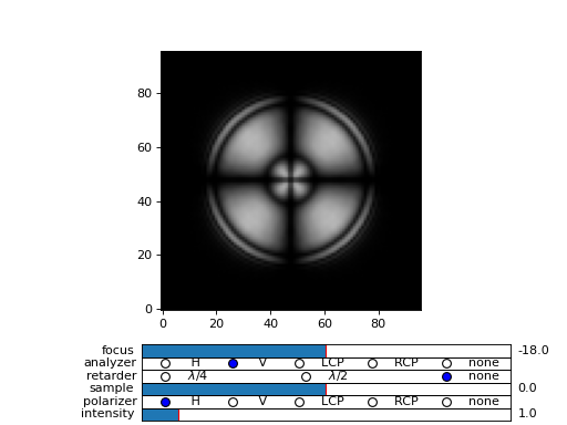
Fig. 34 A hello world example, but this time, with a custom light source and a monochrome camera. (Source code, png, hires.png, pdf)