Quickstart Guide¶

Here you will learn how to construct optical data with the provided helper functions and how to perform calculations for the most typical use case that this package was designed for - propagation of light through a liquid-crystal cell with inhomogeneous director configuration, and visualization (simulation of the optical polarizing microscope imaging). If you are curious about the implementation details you are also advised to read the Data Model first and then go through the examples below. More detailed examples and tutorials are given in the Tutorial.

Importing director data¶

Say you have a director data stored in a raw or text file (or create a sample director data to work with).

>>> import dtmm
>>> NLAYERS, HEIGHT, WIDTH = (60, 96, 96)
>>> director = dtmm.nematic_droplet_director((NLAYERS, HEIGHT, WIDTH), radius = 30, profile = "r")
>>> director.tofile("director.raw")

Here we have generated a director data array and saved it to a binary file written in system endianness called “director.raw”. The data stored in this file is of shape (60,96,96,3), that is (NLAYERS, HEIGHT, WIDTH, 3). That is, a director as a vector defined in each voxel of the computation box. The length of the director vector is either 1, where the director is inside the sphere, and 0 elsewhere. To load this data from file you can use the dtmm.read_director() helper function:

>>> director = dtmm.read_director("director.raw", (NLAYERS, HEIGHT, WIDTH ,3))

By default, data is assumed to be stored in double precision and with “zyxn” data order and system endianness. If you have data in single precision and different order, these have to be specified. For instance, if data is in “xyzn” order, meaning that first axis is “x”, and third axis is “z” coordinate (layer index) and the last axis is the director vector, and the data is in single precision little endianness, do:

>>> director = dtmm.read_director("test.raw", (WIDTH,HEIGHT,NLAYERS,3),
...        order = "xyzn", dtype = "float32", endian = "little")

This reads director data and transposes it from (WIDTH, HEIGHT, NLAYERS,3) to shape (NLAYERS, HEIGHT, WIDTH, 3), a data format that is used internally for computation. Now we can build the optical data from the director array by providing the refractive indices of the liquid crystal material.

>>> optical_data = dtmm.director2data(director, no = 1.5, ne = 1.6)

This converts director to a valid Optical Data. Director array should be an array of director vectors. Length of the vector should generally be 1. Director length is used to determine the dielectric tensor of the material. See Optical Data for details. You can also set the director mask. For instance, a sphere mask of radius 30 pixels can be defined by

>>> mask = dtmm.sphere_mask((NLAYERS,HEIGHT,WIDTH),30)

With this mask you can construct optical data of a nematic droplet in a host material with refractive index of 1.5:

>>> optical_data = dtmm.director2data(director, no = 1.5, ne = 1.6, mask = mask, nhost = 1.5)

Of course you can provide any mask, just that the shape of the mask must mach the shape of the bounding box of the director - (60,96,96) in our case. This way you can crop the director field to any volume shape and put it in a host material with the above helper function.

Note

For testing, there is a dtmm.nematic_droplet_data() function that you can call to construct a test data of nematic droplet data directly. See Optical Data for details.

Sometimes you will need to expand the computation box (increase the volume). You can do that with

>>> director_large = dtmm.expand(director, (60,128,128))

This grows the computation box in lateral dimensions symmetrically, by filling the missing data points with zeros. For a more complex data creation please refer to the Optical Data format.

Note

By expansion in lateral dimension we provide more space between the borders and the feature that we wish to observe. This way we can reduce border effects due to the periodic boundary conditions implied by the Fourier transform that is used in diffraction calculation.

Importing Q tensor data¶

If you want to work with Q tensor data described by a matrix (NLAYERS, HEIGHT, WIDTH ,6), where the 6 components of the tensor are (Q[0,0], Q[1,1], Q[2,2], Q[0,1], Q[0,2], Q[1,2]), there are some conversion functions to use:

>>> Q = dtmm.data.director2Q(director)
>>> Q.tofile("Qtensor.raw")
>>> Q = dtmm.data.read_tensor("Qtensor.raw", (NLAYERS, HEIGHT, WIDTH ,6))

You can convert the tensor to director. This assumes, that you have uniaxial symmetry. If the Q tensor is not uniaxial, the conversion function first makes it uniaxial, by finding the eigenvalues and eigenvectors and determining the most distinctive eigenvalue to determine the orientation of the main axis of the tensor.

>>> director = Q2director(Q)

Alternative approach is to build the epsilon tensor from the Q tensor like

>>> eps = Q2eps(Q, no = 1.5, ne = 1.6, scale_factor = 1.)

Here the scale_factor argument defines the scaling of the effective uniaxial order parameter S. The above function performs $\varepsilon_a = (\varepsilon_e-\varepsilon_o) / s$ where s is the scale factor. The mean value is set to $(2\varepsilon_o + \varepsilon_e)/3.$ . Then dielectric tensor is computed from the diagonal and off-diagonal elements of Q as $\varepsilon = Q_{diag} \varepsilon_a + I\varepsilon_m + Q_{offdiag} \varepsilon_a$ .

Next, we need to convert the epsilon tensor to eigenvalue and Euler angles matrices with

>>> epsv, epsa = eps2epsva(eps)

Alternatively, you can use the convenience function to convert Q tensor to optical_data directly

>>> optical_data = Q2data(Q,no = 1.5, ne = 1.6, scale_factor = 1.)

Transmission Calculation¶

In this part we will cover transmission calculation and light creation functions for simulating optical polarizing microscope images. First we will create and compute the transmission of a single plane wave and then show how to compute multiple rays (multiple plane waves with different ray directions) in order to simulate finite numerical aperture of the illuminating light field.

Plane wave illumination (single ray)¶

Now that we have defined the sample data we need to construct initial (input) electro-magnetic field. Electro magnetic field is defined by an array of shape (4,height,width) where the first axis defines the component of the field, that is, an $E_x$ , $H_y$ , $E_y$ and $H_x$ components of the EM field specified at each of the (y,x) coordinates. To calculate transmission spectra, multiple wavelengths need to be simulated. A multi-wavelength field has a shape of (n_wavelengths,4,height,width). You can define a multi-wavelength input light electro-magnetic field data with a dtmm.illumination_data() helper function.

>>> import numpy as np
>>> WAVELENGTHS = np.linspace(380,780,11)
>>> field_data = dtmm.illumination_data((HEIGHT,WIDTH), WAVELENGTHS, pixelsize = 200, jones = (1,0))

Here we have defined an x-polarized light (we used jones vector of (1,0)). A left-handed circular polarized light can be defined by:

>>> jones = (1/2**0.5,1j/2**0.5)

or equivalently:

>>> jones = dtmm.jonesvec((1,1j)) #performs automatic normalization of the jones vector
>>> field_data_in = dtmm.illumination_data((HEIGHT,WIDTH), WAVELENGTHS, pixelsize = 200, jones = jones)

Warning

The illumination_data function expects the jones vector to be normalized, as it is directly multiplied with EM field coefficients. If this vector is not normalized, intensity of the illumination data changes accordingly.

Most times you need the input light to be non-polarized. A non-polarized light is taken to be a combination of x and y polarizations that are transmitted independently and the resulting intensity measured by the detector is an incoherent addition of both of the contributions from both of the two polarizations. So to simulate a non-polarized light, you have to compute both of the polarization states. The illumination_data function can be used to construct such data. Just specify jones parameter to None or call the function without the jones parameter:

>>> field_data_in = dtmm.illumination_data((HEIGHT,WIDTH), WAVELENGTHS, pixelsize = 200, n = 1.5)

In the field data above we have also used n = 1.5 argument, which defines a forward propagating wave in a medium with refractive index of 1.5. This way we can match the effective refractive index of the optical stack to eliminate reflection from the first surface. With the input light specified, you can now transfer this field through the stack

>>> field_data_out = dtmm.transfer_field(field_data_in, optical_data, nin = 1.5, nout = 1.5)

Here we have set the index matching medium by specifying nin and nout arguments to the effective refractive index of the medium. By default input and output fields are assumed to be propagating in n_cover medium, 1.5 by default.

Note

The transfer_field function by default uses 2x2 method and does not compute reflections. Therefore, nin and nout arguments must be equal. If they are not, you must enable reflections. See Tutorial for details on reflections and interference.

Koehler illumination (multiple rays)¶

If you want to simulate Koehler illumination (see koehler for a nice description of the model) with finite numerical aperture (condenser aperture) multiple rays (or multiple plane waves) needs to be simulated. Directions of these rays have to be defined. A simple approach is to use the illumination_rays helper function. This function returns beta values and phi values of the input rays for a specified numerical aperture of the illumination.

Note

Beta is a sine of ray angle towards the z axis. See Data Model for details.

For numerical aperture of NA = 0.1 you can call

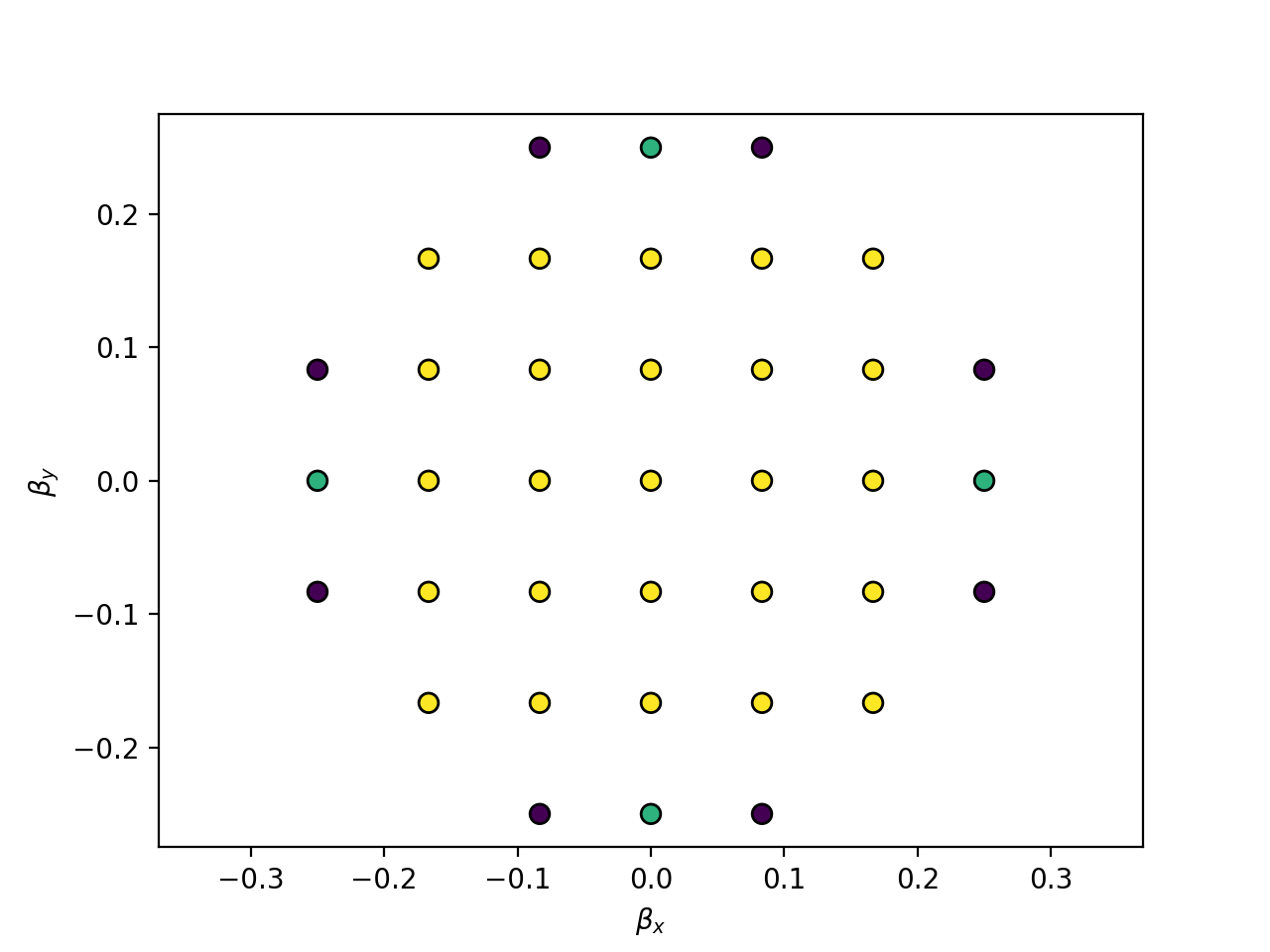
>>> beta, phi, intensity = dtmm.illumination_rays(0.1,7, smooth = 0.2)

which constructs direction parameters and intensity (beta, phi, intensity) of input rays of numerical aperture of 0.1 and with approximate number of rays of Pi*3.5*3.5. It defines a cone of light rays, where each ray originates from a different evenly distributed angle determined from the position of the pixel in a diaphragm of a diameter specified by the second parameter (e.g. 7). Therefore in our case

>>> len(beta)
37

we have 37 rays evenly distributed in a cone of numerical aperture of 0.1.

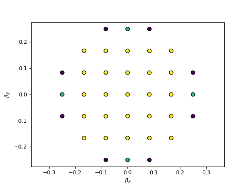
Fig. 2 The beta and beta values of the 37 ray parameters. The color represents the intensity of the ray. (Source code, png, hires.png, pdf)¶

To calculate the transmitted field we now have to pass these ray parameters to the illumination_data and transfer_field functions:

>>> field_data_in = dtmm.illumination_data((HEIGHT,WIDTH), WAVELENGTHS, pixelsize = 200, beta = beta, phi = phi, intensity = intensity, n = 1.5)
>>> field_data_out = dtmm.transfer_field(field_data_in, optical_data, beta = beta, phi = phi, nin = 1.5, nout = 1.5)

Note that we have passed the beta and phi arguments to the transfer_field function, which tells the algorithm that input data is to be treated as multi-ray data and to use the provided values for the ray incidence direction, which is used to determine the reflection/trasnmission properties over the layers. These parameters must match the beta and phi values used in field source creation. Optionally, you can leave the dtmm determine the correct beta and phi, by omitting these parameters and specifying the multiray argument like:

>>> field_data_out = dtmm.transfer_field(field_data_in, optical_data, multiray = True)

Be aware that by default, the illumination_data function creates eigenfields, except if you pass an optional window parameter. Therefore, by default, the beta and phi parameters are approximate values of the true wave vector orientation. See field.illumination_data() for details. Consequently, in reflection calculations in particular, you may face inaccurate calculations resulting from the ill-defined beta values at oblique incidence and at high numerical apertures (the betamax parameter). For an accurate multi-wavelength calculation at oblique incidence use

>>> field_data_out = dtmm.transfer_field(field_data_in, optical_data, multiray = True, split_wavelengths = True)

which treats data at each wavelength as independent, and determines the true incidence angle from the data at each wavelength separately, as opposed to calculating the mean k-vector incidence angle when setting split_wavelengths = False.

Warning

When doing multiple ray computation, the beta and phi parameters in the tranfer_field function must match the beta and phi parameters that were used to generate input field. Do not forget to pass the beta, phi values, or do not forget to specify multiray = True. You are also advised to split the calculation with multi_wavelength argument, for more accurate results.

The dtmm.transfer_field() also takes several optional parameters. One worth mentioning at this stage is the split_rays parameter. If you have large data sets in multi-ray computation, memory requirements for the computation and temporary files may result in out-of-memory issues. To reduce temporary memory storage you can set the split_rays parameter to True. This way you can limit memory consumption (with large number of rays) more or less to the input field data and output field data memory requirements. So for large multi-ray computations do:

>>> filed_out = dtmm.transfer_field(field_data_in, optical_data, multiray = True, split_rays = True)

Note

You can also perform calculations in single precision to further reduce memory consumption (and increase computation speed). See the Configuration & Tips for details.

Microscope simulation¶

After the transmitted field has been calculated, we can simulate the optical polarizing microscope image formation with the POMViewer object. The output field is a calculated EM field at the exit surface of the optical stack. As such, it can be further propagated, and optical polarizing microscope image formation can be performed. Instead of doing full optical image formation calculation, one can take the computed field and propagate it in space (forward or backward) from the initial position. This way, one can calculate light intensities that would have been measured by a camera-equipped microscope had the field been propagated through an ideal microscope objective with 1:1 magnifications. Simply do:

>>> viewer = dtmm.pom_viewer(field_data_out, n_cover = 1.5, d_cover = 0., NA = 0.7, immersion = False)

which returns a POMViewer object for simulating standard objective (non-immersion type) with NA of 0.7. Here we have used the thickness of the cover glass d_cover = 0. This tells the algorithm to neglect the diffraction effects introduced by the thick cover glass. If you have a thick cover glass in the experiment, and you have simulated the field using the transfer_field function with nout = n_cover at the exit surface of the sample, you can use the d_cover argument to simulate aberration effects introduced by the thick cover glass.

Note

For immersion objectives you should specify immersion = True. Here you can use higher NA values. With argument n (defaults to n_cover for immersion objectives) you can specify the refractive index of the output medium (immersion or air).

Warning

You should always match the n_cover argument to that what was used as an output nout refractive index (or input refractive index nin in case you investigate reflections).

Now you can calculate transmission specter or obtain RGB image. Depending on how the illumination data was created (polarized/nonpolarized light, single/multiple ray) you can set different parameters. For instance, you can refocus the field

>>> viewer.focus = -20

The calculated output field is defined at zero focus. To move the focus position more into the sample, you have to move focus to negative values. Next, you can set the analyzer.

>>> viewer.analyzer = 90 #in degrees - vertical direction
>>> viewer.analyzer = "v" #or this, also works with "h","lcp","rcp","x","y" strings

If you do not wish to use the analyzer, simply remove it by specifying

>>> viewer.analyzer = None

To adjust the intensity of the input light you can set:

>>> viewer.intensity = 0.5

The intensity value is a multiplication coefficient for the computed spectra. So a value of 0.5 decreases the intensity by a factor of 0.5.

If input field was defined to be non polarized, you can set the polarizer

>>> viewer.polarizer = 0. # horizontal

You can set all these parameters with a single function call:

>>> viewer.set_parameters(intensity = 1., polarizer = 0., analyzer = 90, focus = -20)

When you are done with setting the microscope parameters you can calculate the transmitted specter

>>> specter = viewer.calculate_specter()

or, if you want to obtain RGB image:

>>> image = viewer.calculate_image()

The viewer also allows you to tune microscope settings dynamically.

>>> fig, ax = viewer.plot()
>>> fig.show()

Note

For this to work you should not use the matplotlib figure inline option in your python development environment (e.g. Spyder, jupyterlab, notebook). Matpoltlib should be able to draw to a new figure widget for sliders to work.

For more advanced image calculation, using windowing, reflection calculations, custom color matching functions please refer to the Tutorial.

Viewing direction¶

If a different viewing direction is required you must rotate the object and recompute the output field. Currently, you cannot rotate the optical data, but you can rotate the regular spaced director field and then construct the optical data as in examples above. There are two helper function to achieve rotations of the director field. If you want to do a 90 degrees y axis rotation you can do:

>>> dir90 = dtmm.rot90_director(director, axis = "y")

This rotates the whole computation box and the shape of the director field becomes

>>> dir90.shape
(96, 96, 60, 3)

This transformation is lossless as no data points are cropped and no interpolation is performed. You may want to crop data and add some border area to increase the size of the computation box and to match it to the original data. Alternative approach, and for a more general, lossy transformation you can use the dtmm.data.rotate_director() function. For a 90 degree rotation around the y axis

>>> rmat = dtmm.rotation_matrix_y(np.pi/2)
>>> dir90i = dtmm.rotate_director(rmat,director)

Now the shape of the output director field is the same, and there are data points in the output that are out of domain in the original data and few data points in the original data were cropped in the proces. The out-of-domain data point are by default defined to be a zero vector

>>> dir90i[0,0,0] #the border is out of domain in the original data, so this is zero.
array([0., 0., 0.])

For a more general rotation, say a 0.3 rotation around the z axis (yaw), followed by a 0.4 rotation around the y axis (theta) and finally, a 0.5 rotation around the z axis (phi), there is a helper function that construct a rotation matrix by multiplying the three rotation matrices

>>> mat = dtmm.rotation_matrix((0.3,0.4,0.5))

It is up to the user to apply a mask or to specify the optical data parameters of these out of domain data points.

>>> mask = dtmm.sphere_mask((NLAYERS,HEIGHT,WIDTH),30)
>>> optical_data = dtmm.director2data(director, no = 1.5, ne = 1.6, mask = mask, nhost = 1.5)

Data IO¶

To save/load field data or optical (stack) data to a file for later use there are load and save functions:

>>> dtmm.save_field("field.dtmf", field_data_out)
>>> dtmm.save_stack("stack.dtms", optical_data)
>>> field_data = dtmm.load_field("field.dtmf")
>>> optical_data = dtmm.load_stack("stack.dtms")

Note

The save functions append .dtmf or .dtms extensions to the filename if extensions are not provided by user.

Increasing computation speed¶

dtmm was developed with efficiency in mind. If you are running on Intel processors, to get the best performance, first make sure you have mkl_fft installed:

>>> import mkl_fft

You can further increase the computation speed. Before loading the package set these environment variables:

>>> import os
>>> os.environ["DTMM_DOUBLE_PRECISION"] = "0" #compile for single precision
>>> os.environ["DTMM_FASTMATH"] = "1" #use the fast math compilation option in numba
>>> os.environ["DTMM_TARGET_PARALLEL"] = "1" #use target='parallel' and parallel = True options in numba

Now load the package

>>> import dtmm

We now have the package compiled for best performance at the cost of computation accuracy. See Configuration & Tips for details and further tuning and configuration options.